The following step-by-step configuration of the Membrane Potential Calibration Wizard is given for the analysis of data recorded by the complete (known kP) calibration potentiometric protocol.
Experimental paradigm for complete calibration with known kP:
1. Baseline: in PM (see protocol) 30 frames
2. Addition #1: stimulation ~ 60min; arbitrary
3. Addition #2: MDC + ASC2 +TTX (see protocol or in Gerencser et al. in J Physiol. 2012 590:12 2845-71) ~ 20 min
4. Addition #3: stir 5 frames, the volume is 150 µl now
5. Addition #4: +10 µl PMK (supplemented with MDC + ASC2 +TTX)
6. Addition #5: +20 µl PMK
7. Addition #6: -40 µl PM +40 µl PMK
8. Addition #7: -75 µl PM +75 µl PMK
9. Addition #8: -100 µl PM + 80 µl PFA in PMK
Steps 1-2 are the actual arbitrary experiment to be calibrated, steps 3-9 are the calibration.
Suggested Pipelines to prepare images for calibration:
Start the Membrane Potential Calibration Wizard from the Tools menu.
1. Calibration Method tab:
1.1. Choose the plasma membrane potential calibration method, e.g. “Complete with known kP (K-steps)”
1.2. Choose the mitochondrial membrane potential calibration method, e.g. “Complete”
2. Input/Output tab: select the input images.
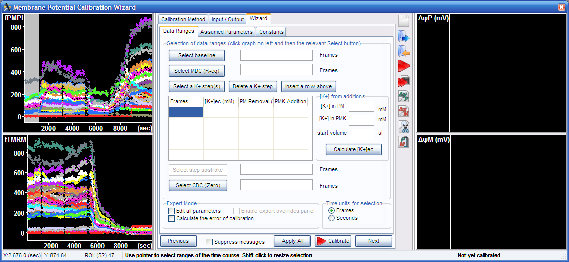
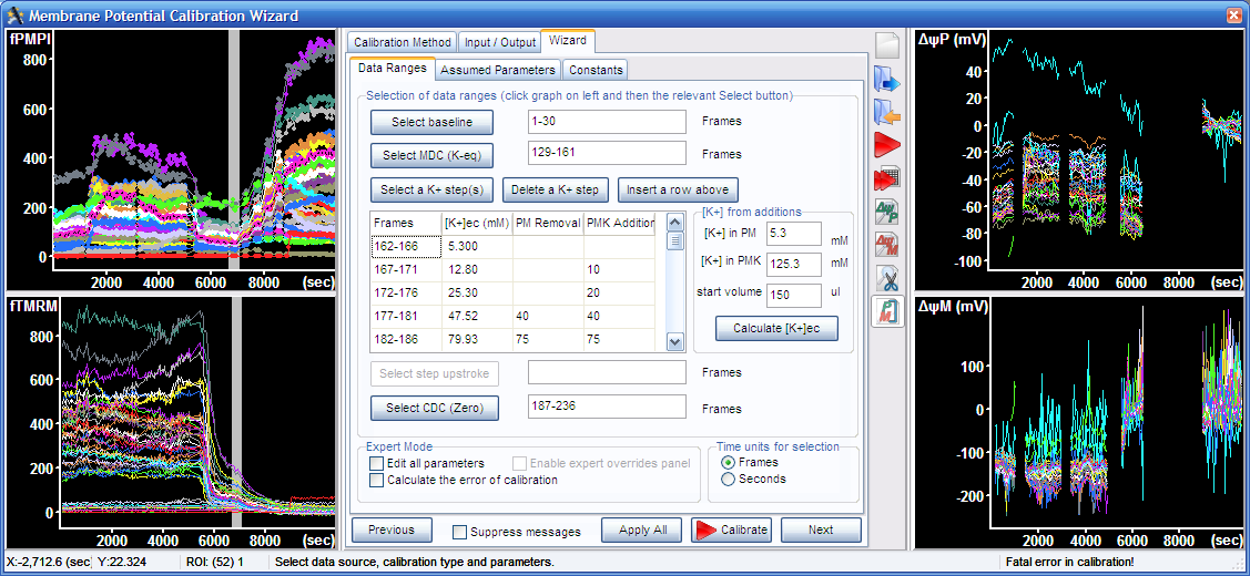
3. Wizard – Data Ranges tab:
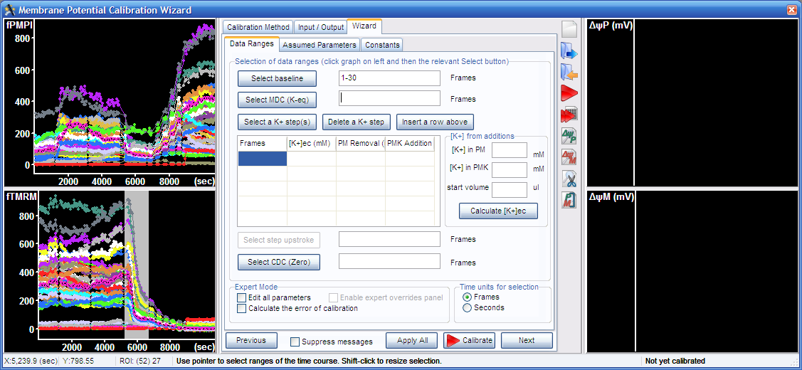
3.1. Select baseline by pointing the range in one of the graphs on the left, and press the “Select baseline button” or alternatively enter the values next to the “Select baseline button”
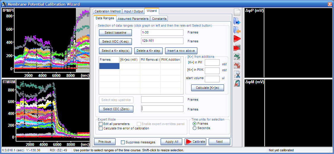
3.2. Select complete mitochondrial depolarization in the graph, and press the “Select MDC (K-eq)” button.
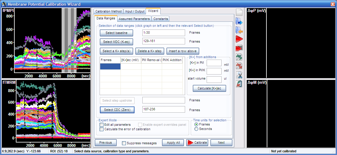
3.3. Select final complete depolarization in the graph, and press the “Select CDC (zero)” button.
3.4. Select the K+-steps, the five segments visible between the mitochondrial and complete depolarization in the top left graph, and press the “Select a K+ step(s)” button.
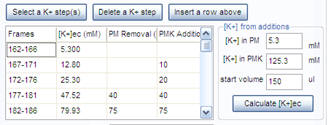
3.5. To calculate [K+] during K-steps, here a tutorial example is described. Enter the K+ concentration in the potentiometric medium (PM), that was 5.3 mM and in the K-based potentiometric medium (PMK), that was 125.3 mM, and the medium volume (150 µl). The K-steps were performed by first adding 10 µl PMK to the assay well. Enter 10 to the second line and “PMK Addition” column in the K-steps table. This was followed by addition of 20 µl (enter it in the next line), then removal of 40 µl and addition of 40ul (in the next line enter 40 to the “PM Removal” column and 40 to the “PMK Addition” column. Finally 75 µl was removed and 75 µl was added (fifth line of the table). Press the “Calculate [K+]ec button”.
4. Wizard – Assumed Parameters tab: No action is required, use the default rate constant for FLIPR redistribution kP=0.38 s-1, and assume no significant non-K-permeability of the plasma membrane during K-steps by using the default PN=0.
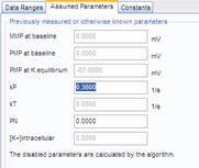
5. Wizard – Constants tab: set the cell specific parameters here:
5.1. VF (mitochondrion:cell volume fraction): use the “Mitochondrion:cell volume fractionator” pipeline to calculate this value using confocal microscopy, assume it based on literature. For the example data set it was measured to be 0.0781 ± 0.0031.
5.2. VFM (matrix:cell volume fraction): this value affects the results only little (because aR’ –see below- largely cancels its effects). The default is 0.8
5.3. aR’ (apparent activity coefficient ratio): use the “Mitochondrial membrane potential assay - measurement of the apparent activity coefficient ratio” pipeline to calculate this value using confocal microscopy. For the example data set it was measured to be 0.360 ± 0.003
5.4. Leave all other constants at their default values.
6. Press
the ![]() Calibrate button
to perform the calibration. Note: not
all cells in the view field can be calibrated, therefore error
messages will appear. Press
cancel to see no
more messages, or check “Suppress messages” in the bottom of the
Calibration Wizard.
Calibrate button
to perform the calibration. Note: not
all cells in the view field can be calibrated, therefore error
messages will appear. Press
cancel to see no
more messages, or check “Suppress messages” in the bottom of the
Calibration Wizard.
7. To
save results press ![]() or
right-click /
”Copy Plot Data” in the graphs on the graphs on the right.
or
right-click /
”Copy Plot Data” in the graphs on the graphs on the right.
8. To explore the results:
8.1. Use
the ![]() and
and ![]() buttons
to see the regression analysis used to calculate calibration
parameters
buttons
to see the regression analysis used to calculate calibration
parameters
8.2. Use
the ![]() button
to see only the time course preceding the calibration steps.
button
to see only the time course preceding the calibration steps.
8.3. Use
the ![]() button
to see only those plasma membrane traces that also were successfully
calibrated for mitochondrial membrane potential. Press
button
to see only those plasma membrane traces that also were successfully
calibrated for mitochondrial membrane potential. Press ![]() again
to refresh the results.
again
to refresh the results.
8.4. Right-click
/ “Calculate Mean” to see mean±SE of
all calibrated traces. To undo mean calculation, press ![]() again. Note: if
the mean calculation is performed on the fluorescence traces on the
left, then the mean data will be calibrated.
again. Note: if
the mean calculation is performed on the fluorescence traces on the
left, then the mean data will be calibrated.
9. Quality control of the calibration:
9.1. Check
“Calculate the error of calibration” in the Data ranges tab within
the Wizard tab and press ![]() .
Now the predicted error of the calibration is shown.Note: optionally,
check the “Suppress messages” on the bottom.
.
Now the predicted error of the calibration is shown.Note: optionally,
check the “Suppress messages” on the bottom.
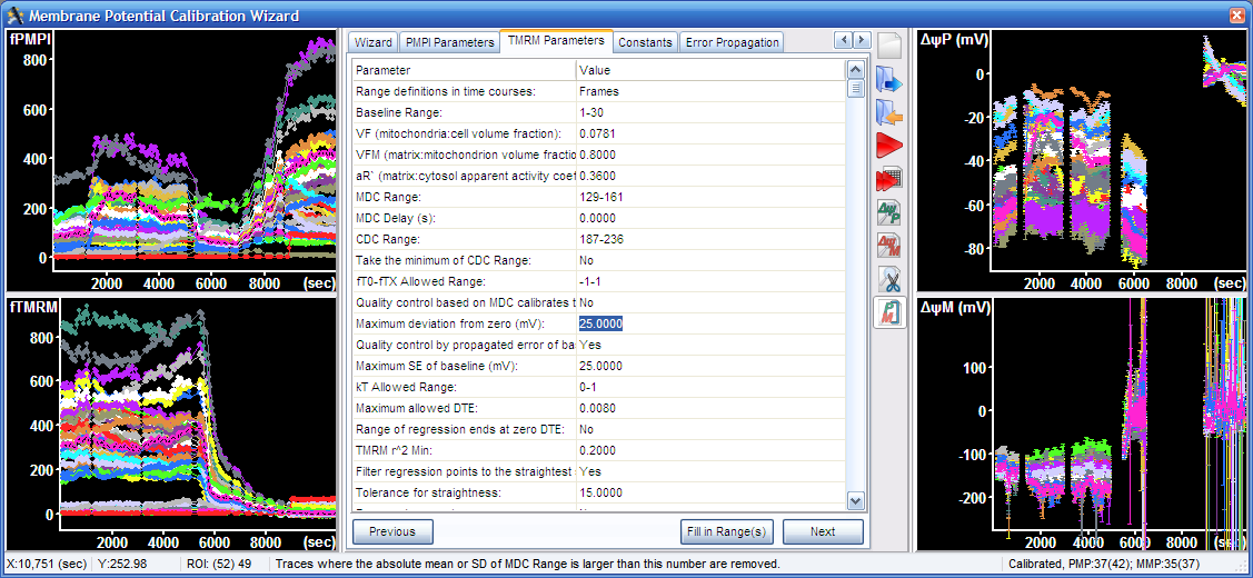
9.2. Check “Edit all parameters”. Detailed lists of all parameters for FLIPR and TMRM calibration, common calibration constants, and error propagation parameters are shown in tabs appearing on the right of the Wizard tab on the top.
9.3. In
the FLIPR parameters, set Quality control by propagated error of
baseline to “Yes” and press ![]() .
Traces with larger predicted error than set at the parameter below
disappear now.
.
Traces with larger predicted error than set at the parameter below
disappear now.
9.4. In
the TMRM parameters, set Quality control by propagated error of
baseline to “Yes” and press ![]() .
Traces with larger predicted error than set at the parameter below
disappear now.
.
Traces with larger predicted error than set at the parameter below
disappear now.
10. Using the Expert Mode: When the Edit all parameters checkbox is checked in the Data ranges tab within the Wizard tab, all parameters of the calibration algorithms can be directly accessed in the tabs appearing on the right of the Wizard tab. These can be used alternatively to the Wizards tab to enter any of the parameters. Use the “Fill in Range(s)” button to automatically enter a range from the selection made in the right graphs.