Fluorescence measurement of mitochondrial swelling in cells

The "ratiometric optimized spatial filtering technique" or "thinness ratio"  (TR) technique measures subtle, subpixel changes of diameters of fluorescent objects in microscopic images. The relative contribution of fluorescence intensities of thinner versus thicker punctate or filamentous structures is measured by a set of two band pass spatial filters. The protocol given below provides a quantitative, single cell, in situ measurement of mitochondrial swelling. The TR decreases proportionally with the increase of the diameter of mitochondria during mitochondrial swelling and is specific to mitochondrial swelling as compared to mitochondrial fission. The technique is sensitive to diameter changes at a 10 nm scale.  The exact description of the technique can be found in Gerencser et al. 2008.

Mitochondrial swelling measurement with the TR technique consists of a calibration recording, looking the effect of valinomycin, and arbitrary number of experiments to be calibrated. The calibration recording is performed per microscopic setting and type of biological specimen (e.g. different fluorphores). Experiments belonging to the same data set have to be recorded under identical microscope settings and processed with the same filter functions to ensure unbiased data.

This protocol assumes that the user is familiar with the following sections of the online manual:

• Spatial filtering in Fourier domain
• Ratiometric Optimized Spatial Filtering .
• Multi-Dimensiona lOpen dialog
• Setup DFT Filter dialog
• Pipeline

Important imaging and specimen requirements:

• TR is calculated from high resolution wide-field or confocal microscopic grayscale images visualizing fluorescently marked mitochondria.
• The specimen must stay completely in focus. Even slight focus drift can cause decaying TR. If the specimen is thick or the focus drifts, use z-stacking.  Thus the thickness and drift determines the number of z-steps, simply to keep the observed mitochondria within the imaged volume. However, TR can be measured in single plane images, if the focus is stabile enough.
• The fluorophore must not redistribute. Therefore membrane potential dyes (TMRM, TMRE, Rh123), Mitotrackers, NOA are unsuitable for TR analysis. Use targeted fluorescent proteins.
• The detector must not be saturated. Edges of saturated areas contain abnormally high frequency components.
• For the fastest analysis use quadrangular, power of two sized images, ideally 512x512.

Recording of the calibration image set

1. Use microscope settings as above given. The calibration and to-be-calibrated recordings must use identical settings.
2. Record baseline for at least 3 time frames
3. Add valinomycin (200 nM) to the sample and when it's swelling-inducing effect is visible record at least further 3 time frames.

Recording arbitrary image sets (experiments)

1. Use the same microscope settings as above. If using different settings (e.g. different magnifications), the calibration has to be performed.

Performing optimization of filter functions on the calibration image set

1. Load the calibration image sequence (download tutorial data set: ).
   1. To z-project XYZT stack the input format must be *.nd, *.nd2 or *.lsm. In the Multi-Dimensional Open dialog Settings tab set Project Z to Mean Intensity. The checkboxes in the Settings tab remain unchecked, unless partial reading of the image stacks is to be performed. For loading non-Multi Time Lapse *.lsm files the z-projection is set in the Preferences Data/Loading/ROIs tab.
   2. For other formats z-project z-stacks before loading into Image Analyst. Use mean intensity projection. If it's not available, use maximum intensity projection. Export as tif-files. Load a set of tif-files into the Image Analyst by multiple selection.
2. Truncate image sequence to contain 3 (or more) baseline followed by 3 (or more) valinomycin treatment frame using the Truncate Image Series . Larger number of frames will take longer time to optimize. In the tutorial data set this is the first and last 3 frames.
3. Draw a ROI encircling mitochondria which stay in focus during the experiment, and the valinomycin-triggered swelling is well visible.
4. Optionally create a mask image. Mask image will improve signal to noise ratio by supressing background. Never use masking on the original image. 
   1. Copy the image, linked.
   2. By using the Segmentation/Threshold function binarize the copy.
      1. Threshold value calculation method: Otsu by frames
      2. Way: Above
      3. Value: 1 (decrease this value to have more mitochondria or increase to have less interference by background noise)
      4. Determine boundaries at: 0 (this number is indifferent here)
      5. Threshold from local max/min: None
      6. Process e.g. by using the context menu of the Image Window.
5. Open the Setup DFT Filter dialog from the Tools main menu
   1. In the Calibration tab enter the Spatial resolution (pixel size) of the image. This can be determined either by pressing Ctrl-I invoking image information in an Image Window, if spatial resolution was saved into the image by the image acquisition software. Alternatively determine it in your image acquisition software. For CCD cameras spatial resolution can be calculated as binning * physical pixel size / lens magnification / any additional zoom, optovar. This value is 0.16 mm/pixel in the tutorial data set.
   2. Note the maximal w, which is calculated from the spatial resolution by the Image Analyst.
   3. In the Optimization tab select the Image to be Optimized. If using mask image, select the mask image as well, otherwise disregard. If the image names do not appear, switch between the Calibration and Optimization tabs back and forth.
   4. At the Select parameters of select Differential Evolution Optimizer. For the tutorial, proceed to next step.
      • The optimizer searches for the filter functions. The default settings result robust optimization of filter functions in mitochondrial swelling assays in cortical neurons and astrocytes imaged at ~0.1 mm/pixel resolution. In the case of misconvergence increase the value for "Population size" or adjust the "Weight" to be a little lower or higher than 0.8. If you increase "Population size" and simultaneously lower "Weight" a little, convergence is more likely to occur but generally takes longer. High values of "Crossover" like 1 give faster convergence if convergence occurs. However, you may have to go down as much as CR=0 to make DE robust enough.
   5. At the Select parameters of select Thinness Ratio Filter Pair. For the tutorial set only the maximum cutoff values (point 2-3 below) and the Use Mask (point 10), and proceed to next step.
      1. The units of spatial frequency is given in cycles/mm as default, but can be changed at the Spatial freq. (ω) unit.
      2. The low band pass (LBP) filter will be searched between LBP minimum cut on ω and LBP maximum cut off ω values typically between 0-1 cycles/mm (see Gerencser et al. 2008 Fig.2.).
         The maximal value must be below the value of maximal w determined at point 5.2 above.
      3. The high band pass (HBP) filter will be searched between HBP minimum cut on ω and HBP maximum cut off ω values typically between 1-3 cycles/mm (see Gerencser et al. 2008 Fig.2.).
         The maximal value must be below the value of maximal w determined at point 5.2 above.
      4. The order of the filter functions (same for all cut ons and cut offs) is searched between Order minimum and Order maximum. Higher order results steeper functions.
      5. Filter normalization: typically corrected integral (see Gerencser et al. 2008 Eq.5,). is used to result intensities at similar order of magnitude after filtering, however as Image Analyst MKII is fully 32bit floating point based, it has little importance.
      6. Test ROI : 1 (if there was only on ROI on the image) Set the number of the ROI to be analysed.
      7. Number of baseline frames: 3 (The image sequence consists of the given number of baseline frames followed by the given number of treated frames. The set of baseline and treated frames can be repeated any time in the same order with the same number of frames to increase the power of the statistics. In the tutorial data set this value is 3. )
      8. Number of treatment frames: 3  (This is the number of frames corresponding to the valinomycin treatment. In the tutorial data set this value is 3.)  
      9. Direction of change: Decreasing (The optimizer can look for  an increasing or a decreasing signal, this is decreasing if valinomycin treatment follows the baseline, as mitochondria are expected to swell and the TR value to decrease.)
      10. Use Mask: Yes if having a separate mask image. No if not. TR will be calculated only at those areas where the mask image has values of '1'.
      11. Preserve edges: No (Performs mirrored tiling to prevent edge artifacts. Slows down processing by 4x. Set it to Yes if interested in details close to the edge of the image.)
      12. Enlarge paper: No  (Enlarges image by mirrored tiling to quadrangular and  prevents edge artifacts and distortions from non-quadrangular images.) Set this to Yes if working on non-quadrangular image.
      13. Enlarge to 2^: 9  Size of image during filtering as power of 2. Used only if Enlarge paper is set to Yes.
      14. Leave only phase: No 
      15. Absolute: Yes
      16. Protect MASK: No (Fills up masked areas and undetermined pixel values with zeros before processing. Required for masked images. In this case the image is not expected to contain masked areas).
   6. Press Optimize, and wait for convergence which can take several (5-10) minutes.
   7. The results for each iteration step are given in the Results box. The results are given as LP or HP cut on-cut off, order; using pixels as spatial frequency units. This avoids the requirement of the image resolution data for further processing. Write down the last pair of LP and HP values.

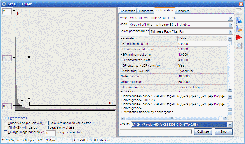The results of the optimization are given in the Results box on the right.

Creating and using a pipeline to perform TR calculation in an arbitrary image set

Mitochondrial Swelling by Thinness Ratio.ips

1. Open a new Pipeline window (main menu Pipeline) and open My Documents/Image Analyst/macros/Mitochondrial Swelling by Thinness Ratio.ips
   1. Click the left 2D DFT Butterworth BP filter in the block diagram, this will be the low band pass (LBP) filter.
      1. Cut On w: enter here the first number after the LP in the results box above
      2. Cut On order and Cut Off order: enter both places the order after the LP in the results box above
      3. Cut Off w: enter here the second number after the LP in the results box above pixels
      4. unit of w: pixels
      5. The rest of the parameters are set identically as it was done in the Optimization/Thinness Ratio Filter Pair above, points 5.5.10-5.5.16. Using Absolute value calculation (Yes) is critical.
   2. Click the right 2D DFT Butterworth BP filter in the block diagram, this will be the high band pass (HBP) filter.
      1. Cut On w: enter here the first number after the HP in the results box above
      2. Cut On order and Cut Off order: enter both places the order after the HP in the results box above
      3. Cut Off w: enter here the second number after the HP in the results box above pixels
      4. unit of w: pixels
      5. The rest of the parameters are set identically as it was done in the Optimization/Thinness Ratio Filter Pair above, points 5.5.10-5.5.16. Using Absolute value calculation (Yes) is critical.
   3. The Threshold in the middle has to set similarly as it was used for masking during optimization
   4. The 2D Nonlinear filters (maximum filters) are necessary for TR image creation. However for plotting only (Ratio Plot) TR data, these filters should be discarded from the pipeline.
      1. To erase 2D Nonlinear filters, unlock editing ,
      2. Right-click 2D Nonlinear filter and select Delete.
      3. Drop The Apply mask by division first on the 2D DFT Butterworth filter, then on the Threshold, to maintain correct order of inputs.
   5. Save the pipeline under a new name.
2. Load an arbitrary image sequence (e.g. the complete image sequence of the tutorial - 9 frames). Use the same kind of projection as for the calibration.
   1. To z-project XYZT stack the input format must be *.nd, *.nd2 or *.lsm. In the Multi-Dimensional Open dialog Settings tab set Project Z to Mean Intensity. The checkboxes in the Settings tab remain unchecked, unless partial reading of the image stacks is to be performed. For loading non-Multi Time Lapse *.lsm files the z-projection is set in the Preferences Data/Loading/ROIs tab.
   2. For other formats z-project z-stacks before loading into Image Analyst. Use mean intensity projection. If it's not available, use maximum intensity projection. Export as tif-files. Load a set of tif-files into the Image Analyst by multiple selection.
3. Process images by running the pipeline using the button.

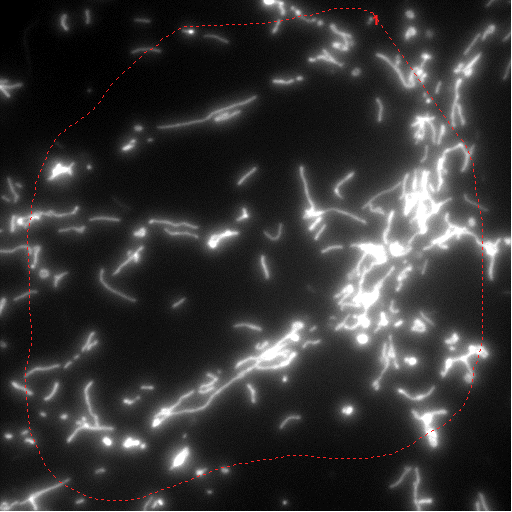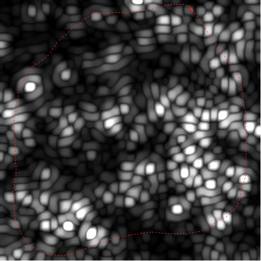
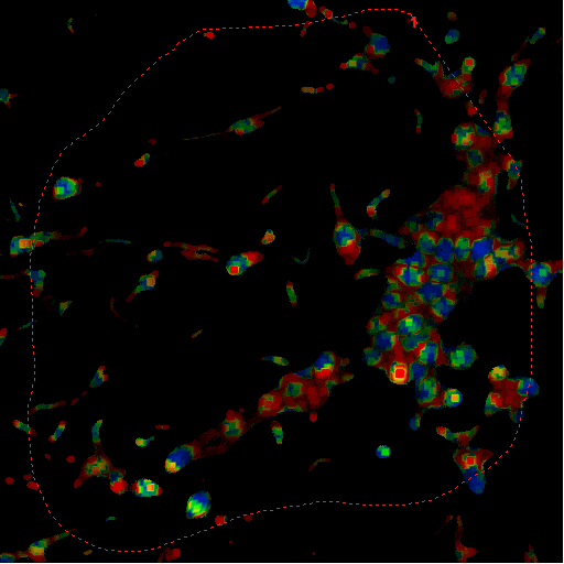
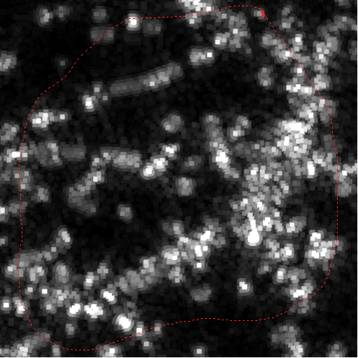
Raw, mean intensity projected image with test ROI	HBP and maximum filtered image before masking	LBP and maximum filtered image before masking
mask image	TR	TR data

Notes:

• TR is insensitive to fluorescence background as long as the cut ons are larger than zero. Therefore no background subtraction is required. 

Protocol by Akos A. Gerencser 02/03/2010 V1.0          

References

1. Gerencser A. A., Doczi, J., Töröcsik, B., Bossy-Wetzel, E., and Adam-Vizi, V. (2008). Mitochondrial Swelling Measurement in Situ by Optimized Spatial Filtering: Astrocyte-Neuron Differences. Biophys J.Sep;95(5):2583-98.