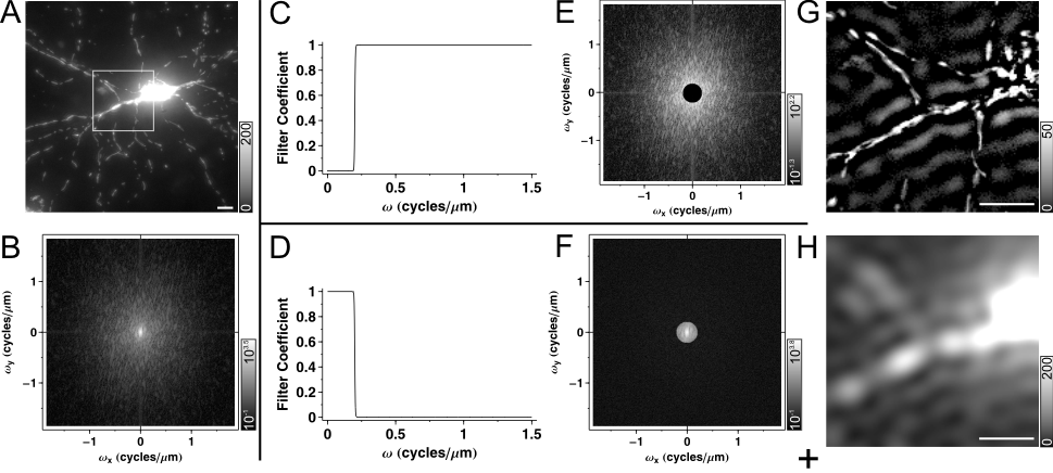
Spatial filtering in Fourier domain is performed by the 2-dimensional discrete Fourier transformation (2D DFT) of the image (Fig. 1A to B), then multiplication of the transform with a 2D transfer function (see below; the product is Fig. 1E) and finally inverse 2D DFT (Fig. 1G). An algorithmic implementation of DFT is the fast Fourier transformation (FFT), but the abbreviations DFT and FFT are often synonymously used. The engineering term for this filtering method is the finite impulse response (FIR) filtering. In 2 dimensions FIR means that when the input of the filtering is a single ‘1’ pixel in an image of zeros (this is the impulse) the result decays to zero in a certain distance from the original ‘1’ (finite response). This response is the point spread function (PSF) of the filter. What is mathematically called convolution in space domain (see kernel convolution filtering) is simplified into multiplication in Fourier domain. The PSF is functionally identical to the kernel in the kernel convolution filtering. The 2D transfer function is therefore the Fourier transform of the convolution kernel.
Image Analyst employs a rotationally symmetric 2D transfer function which is the circumvolution of a filter function (Fig. 1C,D,J) around the origin of the Fourier domain image. This filter function assigns coefficients whether to transmit or reject spatial frequencies 1;2. This implementation specifically manipulates the amplitude information in the image without changing the phase. The effect of multiplication of the Fourier domain image with the rotationally symmetric 2D transfer function is illustrated by Fig. 1E and F. We suggest the specification of filter characteristics in spatial frequency (w) units of cycles/mm (c/mm), because it is independent of the image size or resolution. In the Fourier domain image one pixel of w calibrates to one cycle per physical size of the image (see here).
  |
|
Fig.1. Spatial Filtering in Fourier domain. (A) Maximum intensity projected wide-field fluorescence micrograph of a mito-DsRed2 expressing neuron, a 512´512 image, scaled at 0.27 mm/pixel. Fluorescence intensities were rescaled in the original image to span between 0 and 1000. Images are printed with the indicated gray scaling at g=1.6. Only the region in the rectangle is shown in spatial domain images below. (B) The Fourier domain of (A), shown in a logarithmic scale for better visibility. (C) High pass filter function with a steep, rectangular cut on edge (wcut_on=0.2 cycle/mm). (E) Effect of high pass filtering in Fourier domain and (G) in space domain. Note that the filter function cuts the middle of the Fourier domain with circular symmetry around the origin, and that the steep cut on edge leads to the appearance of ring or halo patterns around bright objects in (G). (D) Low pass filter with a steep cut off (wcut_off=0.2 cycle/mm), complementer of (C), i.e. the sum of the two filter functions is one at each w. (F) Effect of low pass filtering in Fourier domain and (H) in space domain. Because the two filter functions (C and D) are complementers, the sum (I) of images (G) and (H) is identical to the unfiltered image (A). (J-L) High pass filtering with a gradual cut on (J, K; Butterworth filter with wcut_on=0.2 cycle/mm and order=1.5; see 2) mitigates ring formation (K). Using band pass filter with the same cut on provides smoothing or noise suppression (J, L; using a wcut_off=1.2 cycle/mm and order=3). Scale bar, 10 mm. |
The filter function has a biologically meaningful interpretation; can be used for selective transmission or rejection of given sized objects of the image; such as mitochondria (Fig. 1G) or bulkier local background (Fig. 1H). To transmit ~d sized objects, the filter coefficients should be >0 (~1 or greater) for sine wave components with a wavelength l and l/2≈d. To reject objects filter coefficients should be 0 for the given ls.. Because l=1/w, w=1/2d; e.g. 300 nm thick mitochondria will be represented around w=1/(2*0.3mm)=1.67 cycle/mm.
The Fourier domain images above are scaled between ±cycles/(2´pixel size) i.e. at 0.27 mm/pixel resolution (Fig. 1A) between ±1.85 cycles/mm (Fig. 1B,E,F), because for better visualization the origin was placed (both for space and Fourier domain images) into the center of the image. For a comparison, the highest spatial frequency transmitted by a wide-field microscope with an NA=1.3 lens for green light is wmax≈4cycles/mm (see supplementary material of 2). In an exact wording of the Nyquist Sampling Theorem the optimal resolution to completely determine a signal (or image in this case) is at double sampling frequency as compared to the wmax of the optics, thus at 1/(2´2´wmax) ≈1/(2´2´4 cycles/mm) =0.0625mm/pixel in our case.
To perform filtering in Fourier domain we define the following basic filters:
1) A high pass filter function (Fig. 1C-G) with an w=1/(2d) cut on (so the filter function is 1 above this w and 0 below) transmits objects larger and rejects objects smaller than d diameter. However, technically we use band pass filters instead of high pass filters, because the highest spatial frequencies of high resolution microscopic images carry only shot noise, but not image information. Therefore, for noise suppression, it is reasonable to cut down filter functions above the spatial frequencies of the details of the interest (Fig. 1J-L).
2) A low pass filter (Fig. 1D-H) with an w=1/2d cut off (so the filter function is 0 above the cut off w and 1 below) can decrease the contribution of d diameter objects to the image, however due to blur and light scatter fluorescence intensity changes originating from smaller than d-sized objects cannot be completely omitted 1.
3) Filtering with a band pass filter (so the filter function is ~1 between the cut on and cut off ws and 0 otherwise) provides information about the amplitude of the given frequency range (band), or in fluorescent images, yields the intensity of puncti and filaments with a given range of sizes (see below at Ratiometric Optimized Spatial Filtering Technique and in 2).
Spatial filtering in Fourier domain is linear. The order of performing linear transformations does not affect the result. A mathematical property of linearity is that if image a+b=c then this is true for their Fourier transforms and the equality remains true when all three images are spatially filtered with the same filter. Fig. 1A was filtered with a high pass filter (C) resulting (G) and a low pass filter (D) resulting (H). These high and low pass filters were designed to be complementers (their sum is 1 for each w), and filtering with a filter function which is 1 everywhere does not change the image. Therefore the sum of the result images (G+H) provides an identical image (I) to the original one (A, rectangle). Of note, in some of our applications below we use absolute value calculation after spatial filtering, and by this step the linearity is lost.
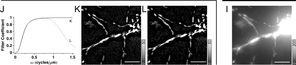
Fourier transformation presumes that the signal (so the image) is cyclic. This means that the image is considered continuous by leaving through right side entering in the left, or leaving through the top entering in the bottom. This has that unfortunate consequence, that if there is a bright object on one edge of the image Fig. 2Ai, it will produce an edge artifact in the Fourier transform (Fig. 2Aii, arrows) and after filtering (Fig. 2Aiii, arrows), on both involved sides of the image. This can be prevented by mirrored tiling Fig. 2B; by creating a twice larger image which is mirror symmetric to its median axes. Then the mirrored-tiled image is transformed, however at four times of computational cost.
 |
|
Fig.2. Prevention of edge artifacts. (Ai) Projection image of a wide-field fluorescence micrograph of a mito-DsRed2 expressing neuron, a 512´512 image, scaled at 0.27 mm/pixel. The Fourier domain (ii) and the result (iii) of high pass filtering with the filter function given in Fig. 1JL are shown. The Fourier domain is visualized in a logarithmic scale. In (iii) only the area corresponding to the white rectangle in (i) is printed. Edge artifacts are indicated by arrows in (ii) and (iii). (B) Edge artifacts are eliminated by mirrored tiling of the spatial image. Note that the number of pixels is doubled in (i) as compared to (Ai) (and also in Fourier domain (ii); not shown), but the scaling of the Fourier domain did not alter (ii). |
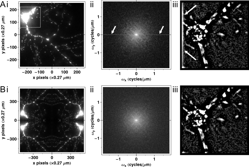
Intensity measurements after spatial filtering in Fourier domain. When low frequency components of an image are removed the remaining higher spatial frequency sine waves fluctuate around zero (Fig. 3A,B), so spatial averaging (like ROI mean calculation) results close to zero mean values. To make regional averaging possible the absolute value of pixels is calculation (Fig. 3C,D). Absolute value calculation also leads to serious ring pattern formation (Fig. 3C), preventing further morphological analysis. Therefore another alternative to substitute zero into every pixel with negative value, i.e. ‘Bottom’ the image at zero.
 |
|
Fig. 3 Negative values in high pass filtered images and absolute value calculation. (A) High pass filtered maximum intensity projection image of a neuron expressing mito-DsRed2. Corresponds to Fig. 1L. (C) The absolute value of (A) was taken. (B,D) Line scan profiles along the dashed white lines in (A) and (B), respectively. Scale bar, 10 mm. |
Relationship to Deconvolution. Our aim here is only to place deconvolution and spatial filtering into the same context. Microscope optics acts as a low pass convolution (or spatial) filter as it forms the image of the sample. Deconvolution is an algorithm to reverse the effects of the convolution by the microscope optics, and improve the image quality. The simplest way of deconvolution is inverse filtering, which is technically high pass filtering with a filter function which is the inverse of the low pass characteristic of the microscope optics. In practice, inverse filtering is strongly impaired by noise, therefore more sophisticated, iterative algorithms are used. Certain image processing procedures detailed below, like dehazing image stacks are in relatively close relation to deconvolution with inverse filtering, therefore we refer to them as empirical 2D blind deconvolution. Acquiring and analyzing time lapses of z-stacks in live specimen have two implications. Firstly, planes of z-stacks are sparsely taken to reduce photo-damage and the time required to image one view-field. In contrast deconvolution needs oversampling both in z and x,y. Secondly, z-stacks have to be processed reasonably fast to enable routine use on larger number of cells / view fields. 2D spatial filtering requires less computation than iterative deconvolution.
Image filtering was performed by Image Analyst MKII, while the Fourier domain image representations were generated by Mathematica (Wolfram Research).
Reference List
1. Gerencser, A. A.; Adam-Vizi, V. Cell Calcium 2001, 30, 311-21.
2. Gerencser, A. A.; Doczi, J.; Töröcsik, B.; Bossy-Wetzel, E.; Adam-Vizi, V. Biophys J 2008, 95(5), 2583-98.