Optical Flow

Optical flow is a measure of sub-pixel dislocations of objects in a time lapse of images. Optical flow is velocity, in a vector or absolute value form, telling for the pixels of an image that how fast and into what direction do the underlying objects move. Optical Flow in fluorescence microscopy can be used for measurement of organelle transport. Because Optical Flow does not depend on object recognition or tracking, but calculated from the dislocation of edges or corners, it can be used for measuring motion to any organelle that is fluorescently labeled, including synaptic vesicles, mitochondria, Golgi and endoplasmic reticule. The velocity measurement is instantaneous or 'snap shot' therefore fusion, fission and overlap of organelles are without effect on the measured velocities. Similarly, the technique is insensitive for new objects entering into the view field or objects lost during a longer time lapse.

This algorithm has been published by Gerencser & Nicholls¹, see details there.

Left: A rat hippocampal neuron expressing mitochondrially targeted GFP (gray outline) was imaged by wide-field microscopy, building an x,y,t,t Multi-Dimensionaldata set in Metamorph. x,y,t,t stands for a time lapse of short time apses. Each short time lapse was processed by Image Analyst MKII resulting an Optical Flow image (pseudocolor overlay). These short time lapses comprised only two frames separated by a one sec interval. The above movie, to show actual velocity vectors, was composed in Mathematica 5.2 from the x and y vector component and the RGB images calculated by the Image Analyst MKII.
Right: A short time lapse of 2 frames, a smaller region of the original 512x512 pixels image is shown. Images are the same recording as on the left side.

Calculation of Optical Flow

Optical Flow is calculated from 'short time lapses' of fluorescence micrographs. The short time lapse in practice means two or more images that were recorded with a short acquisition interval. The short time lapse is optimally two images; two images are sufficient to determine subpixel dislocations of edges of object in the image. Then, a time lapse of Optical Flow (velocity) images can be generated from a time lapse of short time lapses. The 'short time lapse' expression is used to make distinction from the overall time lapse of the the experiment,which comprises of cyclically repeated short time lapses.

Velocities are calculated from the spatial and temporal derivatives of the short time lapse:

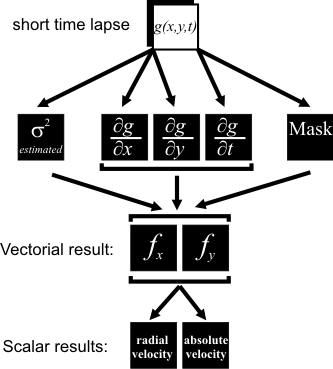
The discrete least squares method of Optical Flow calculation² was reworked for fluorescence microscopy by taking low light level photon shot noise (Poisson noise) in account¹:
Left: The cross section of the edge of an object is shown (blue). g is gray value intensity, x is a spatial coordinate. The object moves to the right. The object was in the light blue position in t1 time point and gets to the dark blue position at t2. Optical flow is calculated over the observed pixel, where the edge of an object passes by. The ratio of the change of the intensity of the observed pixel and the spatial gradient (the steepness of the blue line) gives the velocity. Therefore, when dealing with images, Optical Flow is calculated from the temporally differentiated image sequence (this is the change of intensity in time) and from the spatially differentiated frames (that gives the steepness of the edges).
Right: Simplified scheme of Optical Flow calculation (for details see Gerencser and Nicholls 2008 Figure 7.). A short time lapse (g(x,y,t) referring to gray value intensities according to x,y,t coordinates) is processed by noise estimation (based on known noise characteristics of the camera or detector), by spatial and temporal differentiation, and by binarization. The primary result of the Optical Flow algorithm is a pair of images of the x and y vector components of velocities. Then, absolute velocity, or radial velocity as compared to a point ROI is calculated.

Masking of Optical Flow images

Optical Flow can be unambiguously calculated only where objects have corners, tips, or bent edges. E.g. the motion of a straight, rod shaped object can be determined only at the tips, because it's middle points do not change intensity when it moves along its axis. The Optical Flow algorithm implemented in the Image Analyst MKII masks the images to allow readout of velocities only over those pixels where optical flow can be unambiguously determined.

Image Acquisition paradigms for Optical Flow

The image acquisition requirement of Optical Flow is:

Recording of a short time lapse of two frames with identical imaging parameters (typically ~1 s interval).
The microscope optical parts, stage and focusing mechanism must not move during this short period.
The microscope optical parts, stage and focusing mechanism can move between the short time lapses.
The short time lapses can be combined into complete recordings (experiments) using the following ways (see Figure below):
1. Continuous acquisition over the same position
2. Block mode acquisition over the same position (there is time lag between short time lapses)
3. Multi-Dimensionalacquisition (there is time lag, and motor movement between short time lapses)

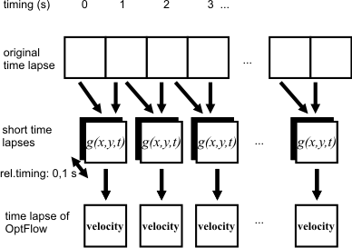
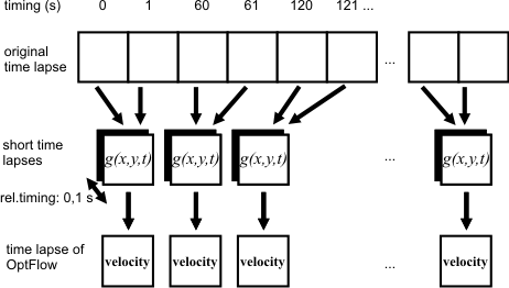
In the Image Analyst MKII a time lapse recording of a single fluorescence channel (recorded either continuously or in block mode), thus the content of an Image Window can be transformed into an Optical Flow (velocity) time lapse (panels A and B below). For this use the Special/Optical Flow function.

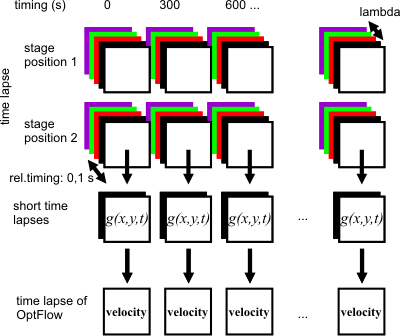
Short time lapses recorded as part of a Multi-Dimensionalacquisition experiment are transformed into an Optical Flow (velocity) time lapse during loading of the selected channel and stage position (panel C, below). This is performed in the Multi-Dimensional Open dialog.

A: Continuous acquisition over the same position: The top row shows frames of the original fluorescence time lapse recording. The bottom row is the resultant time lapse of velocity images. Optical Flow is calculated as running differentiation; the first velocity image from frames 1,2, the second from frames 2,3.

B: Block mode acquisition over the same position: Imaging is paused between short time lapses to decrease photo toxicity

C: Multi-Dimensionalacquisition: each lambda or spectral loop over a stage position is finished by the acquisition of the short time lapse.

References

1. Gerencser A. A. and Nicholls D. G. (2008) Measurement of Instantaneous Velocity Vectors of Organelle Transport: Mitochondrial Transport and Bioenergetics in Hippocampal Neurons. Biophys J. 2008 Sep 15;95(6):3079-99.
2. Jahne, B. 1997. Digital Image Processing. Springer-Verlag, Berlin.