Organelle motion assay with Optical Flow

Optical Flow is a measure of sub-pixel dislocations of objects in a time lapse of images. Optical Flow is velocity, in a vector or absolute value form, telling for the pixels of an image that how fast and into what direction do the underlying objects move (details).

Optical Flow is especially suitable for measuring motion in a Multi-Dimensionalassays, because motion vectors are calculated from pairs of images recorded shortly one after each other. Optical Flow allows visiting multiple stage positions (x,y-coordinates) between time points without an effect of inaccuracies in the stage positioning on the motion. Therefore Optical Flow is discussed in the context of Multi-Dimensionalimage acquisition (e.g. Metamorph Multi-DimensionalAcquisition, Elements ND acquisition, Zeiss LSM Multi Time Series). Image Analyst MKII is an offline analysis tool, therefore relies on recording done by image acquisition softwares.

Requirements for Optical Flow calculation:

1. To calculate Optical Flow pairs of images (short time lapses) are recorded with the same illumination and exposure settings at the very same x,y,z position, with a given time interval.
2. The time points of the acquisition of both images have to be accurately recorded; it is rather important to exactly know the actual time interval between the images than setting accurately a given interval (hardware delays can result altered acquisition intervals).
3. These pairs of images are recorded cyclically, in each time point of the assay, for each stage position. This results a time lapse of short time lapses (see Figure below).
4. Images recorded typically at 512x512 pixels at ~0.2-0.3 mm/pixel resolution. There is no limitation on image size for Optical Flow calculation, but larger images will compute significantly slower.
5. The noise characteristics of the sensor (CCD camera, PMT) has to be measured in a set of evenly illuminated images at different intensities. This must happen at identical camera or PMT settings to the actual experiment.

Setting microscopy parameters

• Wavelength (selection of the fluorophore): Optical Flow analysis is done typically well above the Rayleigh/Nyquist limit, therefore there is no preference between fluorophores of different emission wavelength. In additions velocities/dislocation of edges is not affected by the resolution limit.
• Resolution: For measurement of mitochondrial motion we found that 0.2-0.3 mm/pixel resolution was optimal¹. Higher magnifications may be affected by subtle changes like peristaltic-like motion of inner mitochondrial membrane / cristae, which may not be visually obvious, but generate Optical Flow.
• Acquisition interval: The dynamic range of the Optical Flow is relatively narrow. It measures ~0.1-1.2 pixel/frame velocities (the bottom of the range is determined by the actual signal to noise ratio). Therefore the acquisition interval is determined by the expected velocities the resolution. E.g. if 0.5 mm/s velocities are expected and the resolution is set to 0.2 mm/pixel then the frame interval has to be between 0.1*0.2/0.5=40ms and 1.2*0.2/0.5=480ms. If using short time lapses more than two frames (which is not advised) this time period spans the acquisition from the first to the last frame of the short time lapse.
• Focus: Optical Flow can correctly detect velocities of slightly off focus objects. So if some defocusing happens gradually during a long time lapse that is a little concern. However Optical Flow is highly sensitive for focal changes between frames of the short time lapse. Therefore if active, looped back focusing mechanism is used, it may have to be turned off during the acquisition. Along the same line, it is better to use larger pinhole for Optical Flow acquisitions.
• Stage motors and vibration: Vibration causes uniform error in Optical Flow over the whole image. However in our practice, having microscopes in simple air tables, we did not encounter artifacts accounted for vibration. Some motorized stages with encoders and active loopback may flutter around the set position. Servos should be turned off during Optical Flow acquisition if this is a problem.

Image acquisition

Image acquisition softwares typically do not provide native support for recording a time lapse of short time lapses, with the exception of the Zeiss LSM Multi Time Series module. However, using simple scripting and other 'tricks' short time lapse acquisition can be achieved. This requires individual solutions for each image acquisition environment. Multi-Dimensionalimage acquisition for Optical Flow assays are designed as follows:

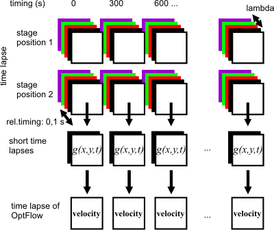Multi-Dimensionalacquisition: each lambda or spectral loop over a stage position is finished by the acquisition of the short time lapse (black and white squares). The reconstituted Optical Flow time lapse for stage position #2 is shown in the bottom. See details here.

Protocols are provided for image acquisition using the systems below, followed by analysis in Image Analyst MKII:

1. Molecular Devices Metamorph 6.3
2. Nikon Elements 3.1
3. Zeiss LSM  Multi Time Series

Analyzing simple time lapse recordings

1. An image series is recorded in an arbitrary image acquisition environment. The timing of each frame has to be accurately saved. There is no stage movement between frames, so all frames perfectly register (if using block mode, fames have to perfectly register within the blocks but not between blocks)
2. An image series loaded as an Image Window can be processed as optical flow.
3. If the recording was not saved as *.stk, *.lsm or *.nd2 file, the import of the timing of the experiment can be problematic. If the acquisition interval was even, the time axis can be entered using the Editing/New Time Scale function.
4. Background must not be subtracted. The original background level is required masking of Optical Flow images.
5. Select the Optical Flow function in the main menu Special are listed. The following parameters may have to be set in the parameter bar:
   1. Select dt kernel: [1,-1] or set the length of blocks if the recording was in block mode.
      • If the block size is greater than 2, set [Savitzky-Golay first derivative] here and enter the size of the block at the SG kernel for dt width, and enter No at #2 below.
   2. Average OF for dt width: Yes (dt kernel of width of two always used with averaging to avoid biasing between leading and trailing edges. Set No if using wider kernel)
   3. Block mode: if the experiment was recorded with an even frame rate around 1s/frame or less set No. If the experiment was recorded as frames (equal number of the width of the dt kernel at short interval, then pause for an arbitrary time, and then this is cyclically repeating, set Yes.
   4. Pixel size: (the mm/pixel calibration can be given here to obtain velocities in mm/s rather than in pixel/s. 1 results output in pixels/s. Use the context menu  Show Image Info of an Image Window to determine scaling)
   5. Output as... (enable the desired kind of outputs; as default only absolute velocities are calculated)
   6. Output as Absolute value of Projected Vectors: If Yes, velocity vectors are projected to a point ROI. This can be used to assess anterograde transport (away from the point ROI) by positive velocities and retrograde transport (towards the ROI) by negative values. When using this feature first (before #3) load the image series by setting the Processing panel to None in the Open tab. Draw ROI on the opened image. Then follow the above protocol form #3. Set the ROI No. in the Projection ROI parameter. The ROIs are automatically copied from the last open image during Optical Flow open.
   7. Other parameters: noise parameters were filled in above. Fine tuning of other parameters see here.
6. In the context menu of the Image Window click Process This with Optical Flow.
7. The default LUT of the Optical Flow image is pseudocolor, and can be set in the Preferences dialog.

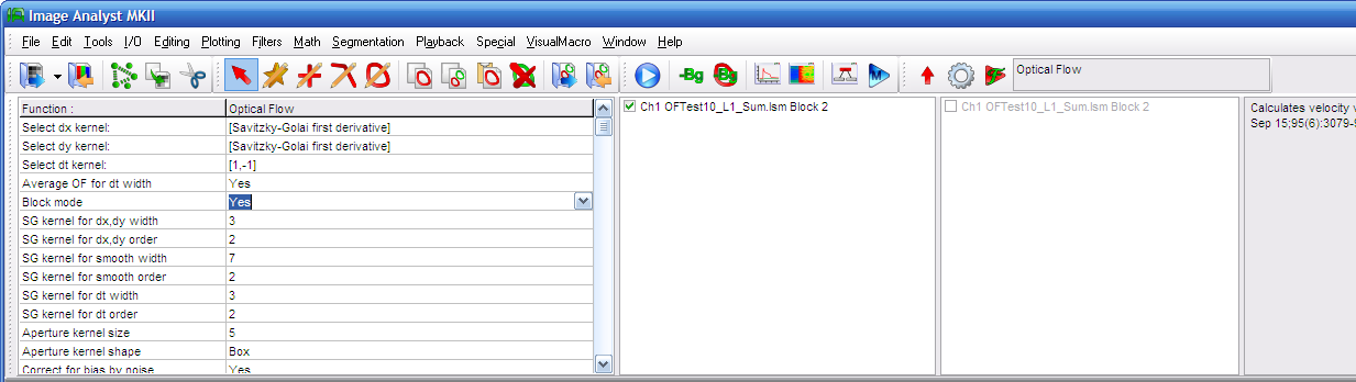Select the Optical Flow function in the Special menu. if the experiment was recorded with an even frame rate around 1s/frame or less set No for the Block Mode. If the experiment was recorded as frames (equal number of the width of the dt kernel at short interval, then pause for an arbitrary time, and then this is cyclically repeating, set Yes for the Block Mode.

Tuning analysis parameters

To perform Optical Flow analysis only the noise parameters, Pixel size and optionally the Block mode have to be set, as given in the detailed protocols (links above), and the rest of the parameters are used at their Default Values. Parameters other than these should be altered only with the understanding the compete Optical Flow algorithm. More about tuning parameters.

See also Working with Optical Flow Images

Protocol by Akos A. Gerencser 11/11/2009 V1.0        

References

1. Gerencser A. A. and Nicholls D. G. (2008) Measurement of Instantaneous Velocity Vectors of Organelle Transport: Mitochondrial Transport and Bioenergetics in Hippocampal Neurons. Biophys J. 2008 Sep 15;95(6):3079-99.