Working with Optical Flow Images
Outputs of the Optical Flow algorithm
- Perform Optical Flow acquisition and loading as detailed
here.
- Output as Absolute value of vectors: pixels
indicate the magnitude of velocity, but not the direction.
- Output as X and Y components of vectors:
results a pair of Image Windows containing the x and y
components of the velocity vectors (because pixel values can be
only scalar)
- Output as Absolute value of Projected Vectors:
Positive velocities indicate movement away from the center point
ROI, negative velocities indicate movement towards the ROI. To
set up the center ROI when using a the Multi-Dimensional Open dialog, first load raw images by
setting the Processing panel to None
in the Open tab. Draw ROI on the opened image. Set the ROI No. in the
Projection ROI parameter. The ROIs are automatically copied
from the last open image during Optical Flow open. Perform
Optical Flow Open.
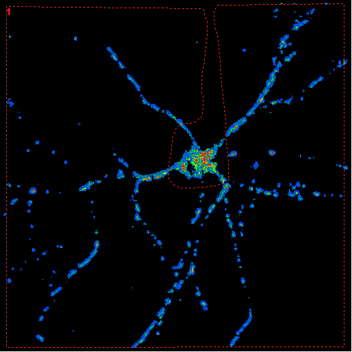
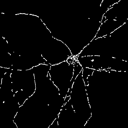
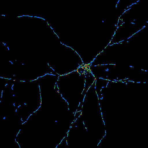
Determining mean absolute velocities of mitochondria
in whole cells
- The example below given on the Metamorph example data set
(download from
here).
- Perform Optical Flow acquisition and loading as detailed
here, by setting the
Output as Absolute value of vectors parameter
Yes, and the other Outputs No.
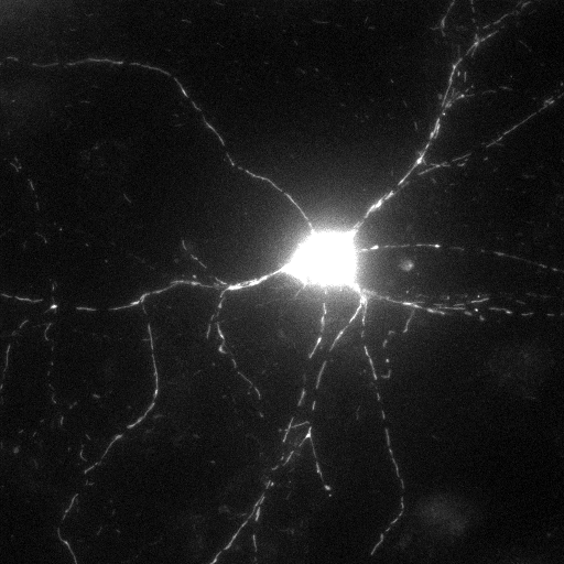
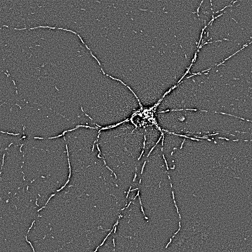
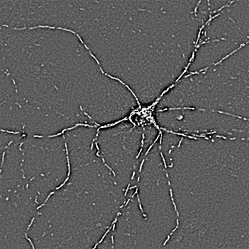
- The non-fluorescent (non-edge) parts of the image are
already masked by the Optical Flow algorithm. Use
 in the toolbar to draw a large ROI
including the whole cell (dendrites of the hippocampal neuron in
the example below) excluding the soma (optionally).
in the toolbar to draw a large ROI
including the whole cell (dendrites of the hippocampal neuron in
the example below) excluding the soma (optionally).
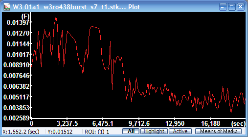
- Press
 in the toolbar to plot mean pixel values, which is absolute
velocity in mm/pixel (as defined by
the Pixel size
parameter)
in the toolbar to plot mean pixel values, which is absolute
velocity in mm/pixel (as defined by
the Pixel size
parameter)
- In some cases additional masking may be required, e.g. to
exclude fast moving 'jumping between frames' mitochondria that
does not result an accurate Optical Flow. In this case masks are
calculated from minimal intensity projections of the short time
lapses. See masking below.
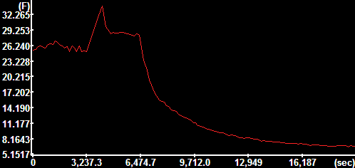
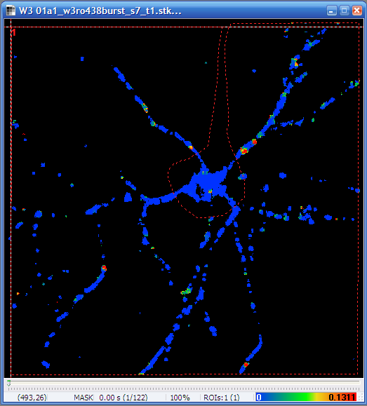 |
 |
| Neuron encircled
without the soma |
Mean absolute
velocity diagram
The y-axis is scaled in mm/sec. |
Processing other channels of the Multi-DimensionalRecording
To obtain graphs of fluorescence intensities in other channels
recorded in each measurement cycle preceding the short time lapse of
the Optical Flow recording:
- Load Optical Flow as above.
- Set Processing in the
Multi-Dimensional Open dialog to None.
- Check all channels (including the (first) Optical Flow
channel)
- Press Open
- In the main menu click
 (Set image windows linkage)
- In the Set image windows
linkage dialog check the name of the Optical Flow Image
Window. Press OK.
- The ROI previously drawn on the Optical Flow image now
appears in the newly loaded Image Windows. To obtain
fluorescence intensities:
- First perform
background subtraction.
- Optionally, perform masking of fluorescence image channels
to look only the same pixels as the Optical Flow image does (see
below).
- Plot each image window by pressing
in the toolbar.
Masking of Optical Flow and other fluorescence
channels
See more about masking here.
Masking using the Optical Flow image:
- Copy (
 Duplicate,
linked) the Optical Flow image. Work on
the copy below.
Duplicate,
linked) the Optical Flow image. Work on
the copy below.
- Select the
 Threshold
function, in the main menu/Segmentation. The
thresholding is set to give 1 for any numerical value in the
image. Mask values automatically result 0.
Threshold
function, in the main menu/Segmentation. The
thresholding is set to give 1 for any numerical value in the
image. Mask values automatically result 0.
- Threshold value calculation method:
Pixel Value
- Way: Above
- Value: If absolute velocity was
calculated give -1. If negative velocities occurr, give a
smaller negative number, e.g. -1000
- Threshold from local max/min:
None (the value of Determine
boundaries at does not apply for None)
-
 Process
e.g. by using the
context menu of the Image Window.
Process
e.g. by using the
context menu of the Image Window.
- Use the Math/Image
Arithmetic function to divide each background
subtracted fluorescence channel by the binarized Optical Flow
image. Division by zero will create the mask.
- Type: /
- Select all of the fluorescence channels as
Image A, and the
binarized copy as
Image B. Press
in the tool bar. Continue working with the results.
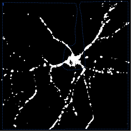 |
 |
 |
| Optical Flow
converted to mask. (Gray scale LUT was applied after the
Threshold) |
High pass filtered
and masked TMRM channel |
TMRM intensity plot |
Using a mask created by locally adaptive thersholding from a
fluorescence image:
- Copy (Duplicate,
linked) the non-processed fluorescence
image. Work on the copy below.
- If working with wide-field microscopy,
perform high pass filtering as
local background removal to amplify mitochondrial details.
- Select the
2D
DFT Butterworth BP filter function, in the main
menu/Filters. Typical parameters are (in cycles/mm;
for this image resoultion have to be present in the file or
set in the
 Setup
DFT Filter):
Setup
DFT Filter):
- Cut On ω: 0.3
(increase this value to make a stronger background
supression, or decrease if the result is too thin, noisy)
- Cut On order: 1.3
- Cut Off ω: 2000
(this is off the scale, so the filter is a high pass filter)
- Cut Off order: 100
- unit of ω: cycles/um
- Filter normalization:
Corrected Integral
- Preserve edges: Yes
- Enlarge paper: No
- Enlarge to 2^:
this value does not matter if above is No
- Leave only phase: No
- Absolute: No
- Protect MASK: No
-
Process
e.g. using the
context menu of the Image Window.
- Smooth image with Wiener filtering:
- Select the
Wiener
filter function, in the main menu/Filters.
- Mask width: 3
- Noise level: 0.0005
(increase this value to increase smoothing)
-
Process
e.g. by using the
context menu of the Image Window.
- Remove values below zero using the bottom
functionality of the
Threshold
function:
- Select the
Threshold
function, in the main menu/Segmentation
- Threshold value calculation method:
Pixel Value
- Way: Bottom
- Value: 0
- Threshold from local max/min:
None (the value of Determine
boundaries at does not apply for None)
-
Process
e.g.by using the
context menu of the Image Window.
- Perform locally adaptive binarization by the
Threshold
function:
- Select the
Threshold
function, in the main menu/Segmentation
- Threshold value calculation method:
Otsu by series
- Way: Above
- Value: 0.5 (decrease this value to have
more mitochondria or increase to have less interference by
background noise)
- Determine boundaries at: 10 (% from
the local maxium for each mitochondrion. Increase this value
to get smaller mitochondria)
- Threshold from local max/min:
Bound Maxima Locally (each object brighter
than the local background by 0.5*Otsu optimal threshold will
be marked down to its 10% of intensity. Note, that if using
high pass filtering, 0% is the full width half max.)
-
Process
e.g. by using the
context menu of the Image Window.
- Use the Math/Image
Arithmetic function to divide each background
subtracted fluorescence channel by the binarized Optical Flow
image. Division by zero will create the mask.
- Type: /
- Select all of the fluorescence channels and the Optical
Flow image as Image A,
and the binarized copy as
Image B. Press
in the tool bar. Continue working with the results.
Note: it is worthwhile to use the
Pipeline for such complex
processing.
 |
 |
 |
 |
| Non-processed,
projection image of the short time lapse. |
High pass
filtered... |
Wiener filtered |
Locally adaptive
binarized |
 |
 |
 |
|
TMRM channel high
pass filtered with similar parameters as above, but with
Absolute: Yes
Shown with 'Fire' LUT |
Masked TMRM image,
shown with Pseudocolor LUT |
(double) masked
Optical Flow Image.
Same frame as shown in the above examples. |
|
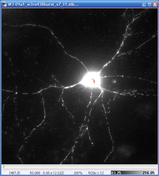
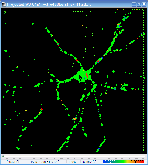
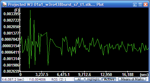
Determining mean radial velocities of mitochondria
in whole cells
- Mean radial velocities carry the information whether
anterograde and retrograde transport is in balance
- Before performing Optical Flow load the non-processed image
sequence by setting the Processing in the Multi-Dimensional Open dialog to None.
- Use the
 point ROI tool to mark the
center of the cell.
point ROI tool to mark the
center of the cell.
- In the Multi-Dimensional Open dialog Processing set
Optical Flow. In the Optical Flow panel set the
Projection ROI parameter as number of the point
ROI.
- Set Output as Absolute value of Projected Vectors:
Yes
- Press Open.
 |
 |
 |
| Non-processed image
with the point ROI in the soma |
Radial velocity
image (note the scaling in the bottom) |
Mean radial
velocity diagram (press Active in the status bar of the
Plot Window to show only the trace of the active ROI).
The y-axis is scaled in mm/sec. |
Determining velocities of individual mitochondria
Velocity measurement of individual mitochondria is based on
segmentation of the same (non-processed) images that is used for the
calculation of the Optical Flow. While
segmentation is discussed
elsewhere in detail. Here we provide an example for robust
segmentation of 'mitochondrial' images. More details here
later...
Using Optical Flow in Pipeline
More details here later...