Recording Optical Flow with the Nikon Elements software

Acquisition in Nikon Elements

Recording noise characteristics

The aim here is to record a set of evenly illuminated fields at different intensities from zero to close to saturation. This have to be performed at completely identical camera settings to the Optical Flow recording.

1. To record noise characteristics use completely identical settings of the camera to the settings used in experiments.
2. Lens and filters do not have to be identical.
3. Mount a fluorescent plastic slide on the microscope. Select a proper optical configuration for the fluorescence spectrum.
4. Focus it to have as even illumination in the image as possible.
   Alternatively the objective lens can be removed and the slide is placed on the nosepiece, in the back focal plane of the lens.
5. Use the Acquire/Capture Time Lapse/Capture Manually feature of Nikon Elements
6. Start with zero illumination; simply acquire an image while the light path is diverted from the camera, e.g. 100% to eyepiece.
7. Set light path to the camera and gradually increase illumination, frame-by-frame. For this:
   1. Use the intensity control of the illumination unit, e.g. Sutter Instruments Smart shutter
   2. or use the aperture diaphragm in the fluorescence illumination pathway
   3. or pull out and then gradually push back the fiber optics light guide
8. It is sufficient to use illumination levels up to it results in similar pixel intensities to the observed intensities during experiments. Do not saturate.
9. Save acquired set (time lapse) of images as nd2 file.

Recording Optical Flow in ND acquisition

The best way for Optical Flow recording in Nikon Elements is to use a repeated channel in the Lambda tab of the ND Acquisition dialog. The following two requirements have to be fulfilled:

1. Accurate timing of Optical Flow frames is required, but Elements does not record time points of the recording of each image within a Lambda loop. However, Elements records the time points of macro command executions, as experiment events. This is set in the Advanced part of the Lambda tab of the ND Acquisition.
2. Sufficient delay has to be applied between acquiring Optical Flow frames. This is achieved by a macro command in the Advanced part of the Lambda tab of the ND Acquisition.

Settings in the ND Acquisition dialog of Nikon Elements

1. Acquisition parameters should result (optimally) 512x512 pixels images at ~0.2-0.3 mm/pixel resolution. For example:
   • 60x lens, 1.0 Zoom, no binning of a 16mm pixel camera: 16/60=0.267 mm/pixel
   • 40x lens, 1.0 Zoom, 2x2 binning of a 6.4mm pixel camera: 2*6.4/40=0.32 mm/pixel
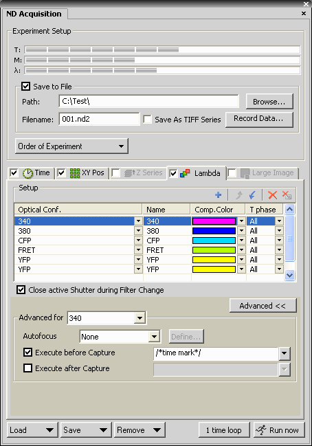
2. Select the Lambda tab of the ND Acquisition dialog
3. Set up channels (optical configurations) to be acquired. The channel used for Optical Flow measurement is added twice as the two last channels.
   The channel used for Optical Flow is simply the optical configuration of the fluorophore that visualizes the moving organelle, e.g. mito-GFP.
4. Because the Optical Flow calculation depends on the noise parameters of the camera, the gain, multiplier, AD conversion clock (MHz) settings (if applicable for the camera in use) should not be varied between experiments, unless the noise characteristics is measured for each setting. The exposure time may be varied. The safest to set intensities by varying illumination intensities.
5. Open the Advanced part of the dialog
6. For each channel (optical configuration used), check the Execute before capture checkbox, and enter a commented expression e.g. /*time stamp*/
   Commenting is done by slash-star star-slash bracketing. The comment text has to be identical for all channels, this will be detected by the Image Analyst. If using other macro commands, these can precede or follow the comment, e.g. when using macro commands to offset focus compensating for chromatic aberration.
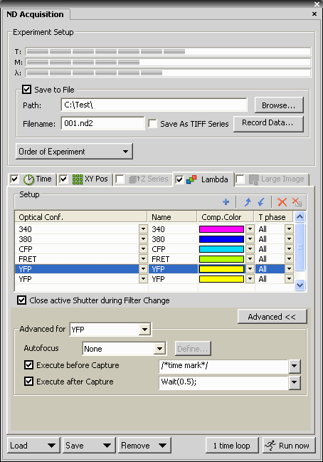
7. For the first channel used for Optical Flow check the Execute after capture checkbox, and type: Wait(0.5);
   This sets up the interval between the two Optical Flow images. The interval is given in seconds, and there is also a significant hardware delay that adds to this delay. The value of 0.5 is an example here, it has to be set according the application (see Gerencser & Nicholls 2008). To determine real frame interval, use Image Analyst MKII, In the Multi-Dimensional Open dialog, set:
   1. Open/Processing/Single Time Point
   2. ND2 Tweak/Use events for experiment timing... and Load multiple channels as Z or OF
   3. Load a time point and look for the timing in the status bar of the Image Window.
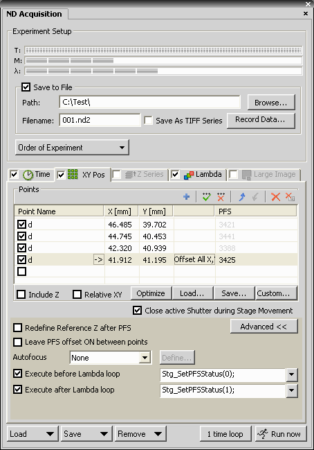
8. The Time and XY Pos tabs can be arbitrarily set, while the Z-Series and Large Image are disabled.
9. It is advised to use the perfect focus system (PFS), or other means of software auto focusing, if PFS is not available.
10. If using PFS, it may be turned off for the duration of the acquisition of the Optical Flow frames, to ensure that no focal change happens due to fluttering of the active feedback mechanism of the PFS.  To turn it off change the Execute before capture command of the first Optical Flow channel to  /*time stamp*/Stg_SetPFSStatus(0);

In this example cells are stained by Fura-2-AM and expressing mitochondrially targeted cameleon. Add the same comment e.g. /*time stamp*/ to each channel Execute Before Capture.	The last channel (YFP) is repeated once, so the two YFP channels will be used for Optical Flow calculation. At the first Optical Flow channel set the Execute After Capture to Wait(0.5); Use the proper wait time. Expect a significant hardware delay in addition to the exposure time.	If using the perfect focus system: In the XY Pos tab set:  Execute before Lambda Loop: Stg_SetPFSStatus(0); to turn PFS off Execute after Lambda Loop: Stg_SetPFSStatus(1); to turn PFS on

The protocol is based on Nikon Elements AR 3.0 and 3.1.

Analysis in Image Analyst MKII

Analyzing noise characteristics

1. Open the noise characteristics file recorded above
2. Set LUT scaling to frame-by-frame in the Set scaling menu point of context menu of the Image Window (check Scale each frame independently)
3. Look for a small part of the image where the illumination is the most even. Draw a small ROI here (~20x20 pixels)
4. Select the Sensor Noise Characteristics in the Special main menu.
5. In the Parameter Bar, set the 'Set values in Optical Flow functions' parameter to Yes.
6. In the context menu of the Image Window click Process This with Noise Characteristics; A Plot and a Text window appear.
7. The content of the Plot window is the intensity-variance relationship of the pixels within the ROI. This has to be a straight line. If it is not linear:
   1. Frames have to be in the order of increasing intensity
   2. Delete any saturated frames.
   3. Nonlinearity may be caused by uneven illumination. Move the ROI around to find a linear spot.
   4. Try to draw a smaller ROI.
8. The function automatically sets the following parameters of the Optical Flow function:
   • Detector offset (mean of the zero illumination image intensity)
   • Detector variance vs. intensity Slope (slope of the Plot Window)
   • Detector Read out Variance (variance at the zero  illumination)
9. The above values will be stored when exiting Image Analyst, or click Edit/Save Preferences in the main menu.

Noise curve of a Cascade 512B CCD camera at binning: 1x1; Exposure: 100 ms; Multiplier: 2100; Readout Speed: 5 MHz; Conversion Gain: 1/3 x; Temperature: -30.1°C The image on the left was scaled between its 1 and 99 percentiles, therefore shows inhomogeneities amplified. Of note the readout noise show on the right is higher than typical for this camera type, because of improper Multiplier and Gain settings...		Offset: 1,317.0 Variance vs. intensity Slope: 1.9810 Readout noise (variance σ2): 201.51 --------------------------------------------------- Electrons per gray unit: 0.5048 Readout noise (e-;RMS): 10.086

Analyzing Optical Flow

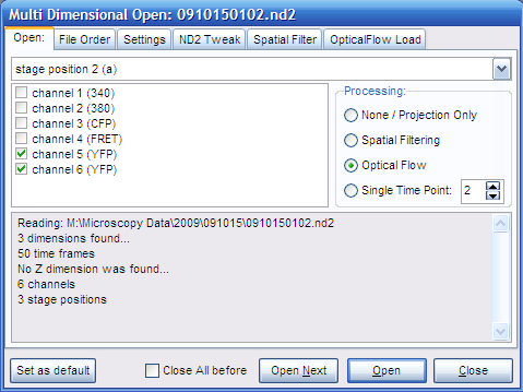
1. Open the ND Acquisition file (*.nd2). If the experiment consists multiple *.nd2 files they can be merged in time by multiple selection. The Multi-Dimensional Open dialog appears.
2. In Open tab: select only the two channels that will be used for Optical Flow calculation. Select Optical Flow in the Processing panel.
3. In the Settings tab make sure that the Load specified frames of each stack... and the Separate Blocks... are not checked. The Load specified frames of the time lapse feature can be used. If more frames are processed than the width of the dt (temporal differentiation) kernel, multiple velocity images are calculated, and the result will be obtained by using projection as given in the Project Z field.
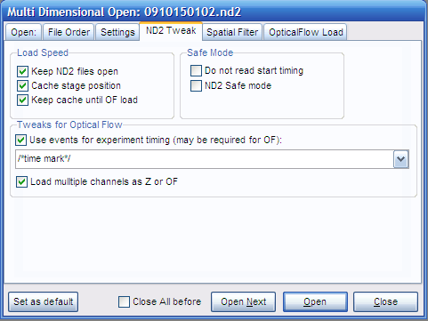
4. In the ND2 tweak tab: check the Use events.... This feature is available only if macro command / comment events were properly assigned before ND acquisition in the Elements. Select below the actual time stamp, e.g. /*time stamp*/. Also check Load multiple channels as Z or OF.
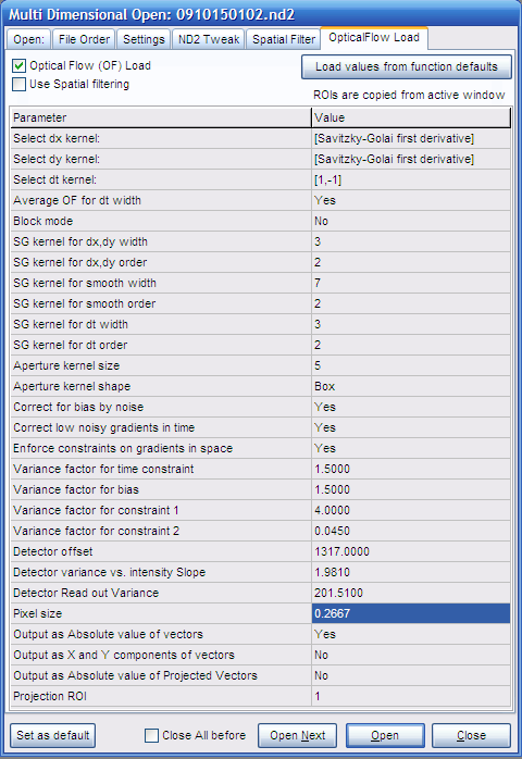
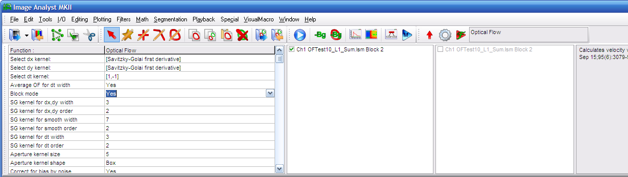
5. In the OpticalFlow load tab the parameters of the Optical Flow function are listed. The following parameters may have to be set here:
   1. Select dt kernel: [1,-1]  (to match the length of short time lapses of two frames)
      • If the block size is greater than 2, set [Savitzky-Golay first derivative] here and enter the size of the block at the SG kernel for dt width, and enter No at #2 below.
   2. Average OF for dt width: Yes (dt kernel of width of two always used with averaging to avoid biasing between leading and trailing edges)
   3. Block mode: No (each short time lapse is separately processed, so there is no need for block mode)
   4. Pixel size: (the mm/pixel calibration can be given here to obtain velocities in mm/s rather than in pixel/s. 1 results output in pixels/s.  Use the context menu  Show Image Info of an Image Window, or the Tools/Setup DFT filter to determine scaling)
   5. Output as... (enable the desired kind of outputs; as default only absolute velocities are calculated)
   6. Output as Absolute value of Projected Vectors: If Yes, velocity vectors are projected to a point ROI. This can be used to assess anterograde transport (away from the point ROI) by positive velocities and retrograde transport (towards the ROI) by negative values. When using this feature first (before #2) load the image series by setting the Processing panel to None in the Open tab. Draw ROI on the opened image. Then follow the above protocol form #2. Set the ROI No. in the Projection ROI parameter. The ROIs are automatically copied from the last open image during Optical Flow open.
   7. Other parameters: noise parameters were filled in above. Fine tuning of other parameters see here.
6. Above settings are valid as long as the dialog is open, or can be stored by the Set as Default button.
7. Click Open to perform loading and processing.
8. The default LUT of the Optical Flow image is pseudocolor, and can be set in the Preferences dialog.

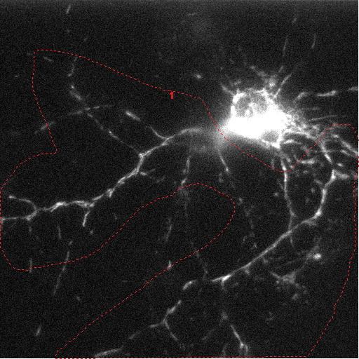
The resultant Optical Flow image consists of pseudocolored pixels where Optical Flow determination was feasible based on the noise characteristics (there was enough image detail to distinguish movement from noise), and black mask where not. The unit of the Optical Flow image is pixel/s, or mm/s  if the Pixel size is set above.

	Setting the /*time stamp*/ and checking Load multiple channels as Z or OF are crucial for Optical Flow processing. However uncheck the Load multiple channels as Z or OF  if loading channels for analysis of fluorescence intensity.

Analyzing Optical Flow from simple time lapse recordings (see figure about block mode)

1. Open nd2 file in the File/Open image series/measurement, and in the Multi-Dimensional Open dialog load the complete time lapse by setting the Processing to None.  Importantly, this section is only valid for time lapses recorded without stage movement.
2. Background must not be subtracted. The original background level is required masking of Optical Flow images.
3. Select the Optical Flow function in the main menu Special are listed. The following parameters may have to be set in the parameter bar:
   1. Select dt kernel: [1,-1] or set the width of blocks if the recording was in block mode.
      • If the block size is greater than 2, set [Savitzky-Golay first derivative] here and enter the size of the block at the SG kernel for dt width, and enter No at #2 below.
   2. Average OF for dt width: Yes (dt kernel of width of two always used with averaging to avoid biasing between leading and trailing edges. Set No if using wider kernel)
   3. Block mode: if the experiment was recorded with an even frame rate around 1s/frame or less set No. If the experiment was recorded as frames (equal number of the width of the dt kernel at short interval, then pause for an arbitrary time, and then this is cyclically repeating, set Yes.
   4. Pixel size: (the mm/pixel calibration can be given here to obtain velocities in mm/s rather than in pixel/s. 1 results output in pixels/s. Use the context menu  Show Image Info of an Image Window to determine scaling)
   5. Output as... (enable the desired kind of outputs; as default only absolute velocities are calculated)
   6. Output as Absolute value of Projected Vectors: If Yes, velocity vectors are projected to a point ROI. This can be used to assess anterograde transport (away from the point ROI) by positive velocities and retrograde transport (towards the ROI) by negative values. When using this feature first (before #3) load the image series by setting the Processing panel to None in the Open tab. Draw ROI on the opened image. Then follow the above protocol form #3. Set the ROI No. in the Projection ROI parameter. The ROIs are automatically copied from the last open image during Optical Flow open.
   7. Other parameters: noise parameters were filled in above. Fine tuning of other parameters see here.
4. In the context menu of the Image Window click Process This with Optical Flow.
5. The default LUT of the Optical Flow image is pseudocolor, and can be set in the Preferences dialog.

Select the Optical Flow function in the Special menu. if the experiment was recorded with an even frame rate around 1s/frame or less set No for the Block Mode. If the experiment was recorded as frames (equal number of the width of the dt kernel at short interval, then pause for an arbitrary time, and then this is cyclically repeating, set Yes for the Block Mode.

Fine tuning optical flow (see here)

Example

Example nd2 file (43MB, zip compressed)
Download and uncompress data on your hard drive.

1. In the main menu select File/Open image series/measurement, set the file type to "*.nd2"  and open noise.nd2 in the “Noise Characteristics” folder.
2. Press Open in the appearing Multi-Dimensional Open dialog.
3. Discard the last 3 frames because of saturation using the toolbar icon.
4. Follow the points in the Analyzing noise characteristics section above.
5. Close images by File/Close all.
6. In the main menu select File/Open image series/measurement, set the file type to "*.nd2" and select the file in the “Mitochondrial Motion” folder.
7. Set ND2 Tweak and and Optical Flow tabs as shown above (the noise parameters should be automatically entered by now)
8. In the Settings tab uncheck everything.
9. Switch back to the Open tab, select stage position 3 and only the two YFP channels and Click Open. Inspect images.
10. The Pixels size can be obtained in the Tools/Setup DFT Filter dialog.
11. Select Optical Flow in Processing and press Open again.
12. Draw a ROI around the neuron and press .
13. To analyze the Ca²⁺-imaging channels, first go back to the ND2 Tweak tab and uncheck Load multiple channels as Z or OF
14. In the Open tab select Processing None and the first four channels. Click open.
15. Click and subtract background of the intensity images at 5 percentile from all images.
16. Click to link intensity image to the already open Optical Flow image.
17. Use the Math/Ratio to obtain Fura-FF 340/380 ratio or cameleon FRET/CFP ratio. Proper FRET calculation from this data needs spectral unmixing.

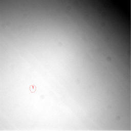
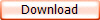
Frame 1 of projection image of stage position 3 Hippocampal neuron expressing mito-D4cpv targeted cameleon, acquired by a Nikon Ti2000 PFS	Frame 1 of Absolute Velocity Image	Mean absolute velocity over the encircled area in the images. The y-axis is scaled in mm/sec.

Protocol by Akos A. Gerencser 08/10/2010 V1.1        

References

1. Gerencser A. A. and Nicholls D. G. (2008) Measurement of Instantaneous Velocity Vectors of Organelle Transport: Mitochondrial Transport and Bioenergetics in Hippocampal Neurons. Biophys J. 2008 Sep 15;95(6):3079-99.