Measurement of velocities and fluorescence intensities over single mitochondria

This protocol describes how to segment fluorescence time lapse image sequences to determine velocities and other parameters of individual mitochondria, like intensities of other fluorescence channels, size and length. The technology described here is an improved version of our earlier described method.  The protocol consists of the preparation of images for segmentation (local background removal, smoothing), segmentation and reading out values corresponding to segments. Measurement of anterograde and retrograde or directional vs. wiggling motion is given at the bottom.

This protocol assumes that the user is familiar with the following sections of the online manual and protocols:

• Organelle motion assay with Optical Flow
• Spatial filtering in Fourier domain
• Binarization, Thresholding, Segmentation
• Segmentation of images
• Pipeline

Protocol for segmentation

• If using  Multi-Dimensional Open dialog:
  • Load the original (raw) fluorescence time lapse image sequence with minimum intensity projection (Settings tab). Minimum intensity projection is used to show only those mitochondria that move slowly, thus the Optical Flow and intensity readouts will be correct.
  • Optionally, subsequently, load other channels, if present, e.g. the TMRM channel in the example below.
  • Perform Optical Flow load as described in the "Organelle motion assay with Optical Flow".
• If using simple time lapse recordings, load the original (raw) fluorescence time lapse image sequence.
  • Create a copy of the image.
  • Perform Optical Flow on the copy as described in the "Organelle motion assay with Optical Flow".
  • Rename the resultant image to 'Optical Flow' (Main menu/Edit/Rename).
  • Project the original image with the Filters/Temporal block filter / Filter type=Min / Window width = the value of SG kernel for dt width or 2 if dt kernel=[1,-1] for the Optical Flow calculation. The value of Block mode is identical to the Block mode of the Optical Flow. Minimum intensity projection is used to show only those mitochondria that move slowly, thus the Optical Flow and intensity readouts will be correct.
  • Link images with .
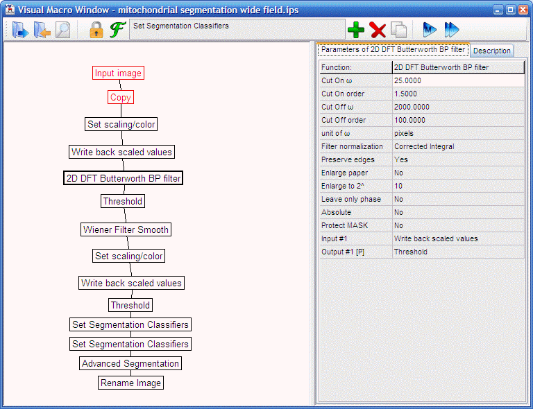
• Load the "mitochondrial segmentation wide field.ips" , select the minimum intensity projection image and use the to run it (the steps of the pipeline are detailed below, in routine use proceed to the next step):

1. Set scaling/color and Write back scaled values: values between 0-99.99
2. 2D DFT Butterworth BP filter: 25/1.5/2000/100/pixels/.../absolute=No : this is a highpass filter with a cuton at 25 pixels spatial frequency to show mitochondria only. Note that if images with different size or spatial resolution are to be processed, a different cuton frequency will be required. See more in "Spatial filtering in Fourier domain" and in "Background removal by highpass filtering". The spatial frequency value of 25 pixels is 0.175 cycles/mm at 512x512 images at 0.28 mm/pixel resolution in the example shown below. The 0.175 cycles/mm is a constant value for mitochondrial filtering. So if using different image size or resolution, set the spatial resolution in the Tools/Setup DFT Filter dialog Calibration tab, and either calculate the new cut on spatial frequency in pixels as 0.175/w resolution (w resolution is displayed below the spatial resolution) or set the 2D DFT Butterworth BP filter the unit of w parameter to cycles/mm.
3. Threshold: Bottom at Pixel value = 0 (Threshold from local max/min=None): this removes negative values created by the high pass filter.
4. Wiener Filter Smooth: adaptive filter for noise removal. Increase noise level for stronger noise removal. Decrease noise level if mitochondria are smudged.
5. Set scaling/color and Write back scaled values: values between 0-99.85. The Max percentile 99.85 sets the sensitivity of the segmentation operation below. Increase this value to have fewer segments. Decrease this value to have more segments.
6. Threshold: Mask below Pixel value = 100 (Threshold from local max/min=None): this suppresses background. Increase this value if mitochondria look overflowing.
7. Set Segmentation Classifiers: Limit Type=Max: segments with parameters larger than the given values are rejected (erased from the image). Zero means that the given parameter is not looked. (no classifiers are set in the example)
8. Set Segmentation Classifiers: Limit Type=Min: segments with parameters smaller than the given values are rejected (erased from the image). Zero means that the given parameter is not looked. (no classifiers are set in the example)
9. Advanced Segmentation: Otsu by Series, Above, at 1, Threshold from local max/min=Bound locally, Determine boundaries at 10%), Method=Watershed, Connectivity=Inf. This performs local maximum search and segmentation with the combination of locally adaptive thresholding and the watershed algorithm. In the segmented image segments are marked with different values and frames are independent from each other.
10. Rename Image to "Segments"

• Showing and Exporting data (manually execute procedures, or program it into Pipeline)

1. Select Plotting/Plot Intensities Corresponding to Segments: Type=Mean, all other parameters are No.
2. Select the image "Segments" as  Image A. Select the Optical Flow image (or any of the intensity images) as Image B and press process in the tool bar. A plot window appears with circles indicating values in Image B in overlapping pixels for each segment of Image A. Segments are independent between frames (i.e. are not tracked), therefore the Time Continuous Segments parameter was set to No. The y-axis is labeled with 'F' regardless the modality/unit of the measured quantity. If not all images appear as Image B, use the link tool.
3. Use the context menu (right click) of the Plot window to save or copy data. If data is copied to Excel, beware that Excel will handle only 253 columns, so segments.

• Constraining segment evaluation to a ROI

1. Draw a region ROI (on any of the images because all are linked by this time) with the toolbar button, encircling some of the segments.
2. In the Plotting/Plot Intensities Corresponding to Segments and change the Constrain to Active ROI parameter to Yes.
3. Perform plotting as above.

• Working with exported velocities
  • Image Analyst MKII does not support statistical evaluation of fluorescence or velocity data, therefore data is exported as TAB delimited text file or by clipboard copy/paste operation from the Plot Window.
  • Use a statistical software capable of calculating histograms and importing TAB delimited text files transposed (e.g. Graphpad Prism or Sigmaplot)
  • To determine number (or percentage) of fast moving or stationary mitochondria calculate histograms. Mitochondrial velocities typically show continuous distribution, therefore the threshold between stationary and moving mitochondria has to be arbitrarily determined.

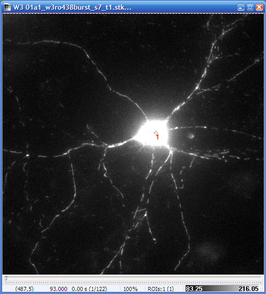
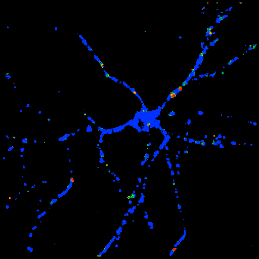
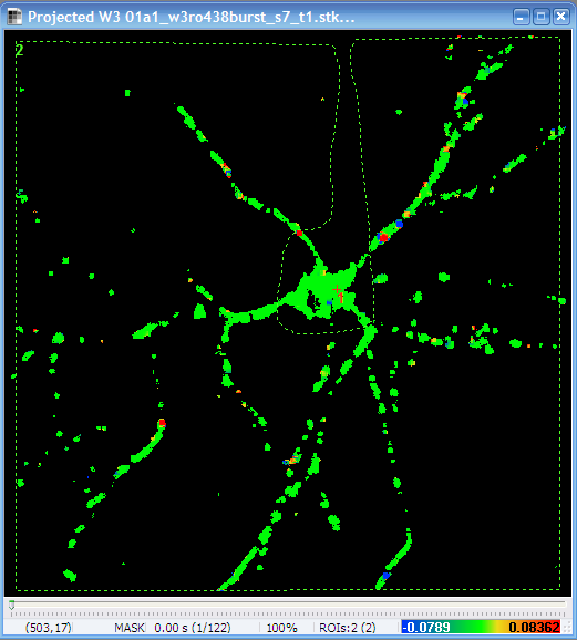
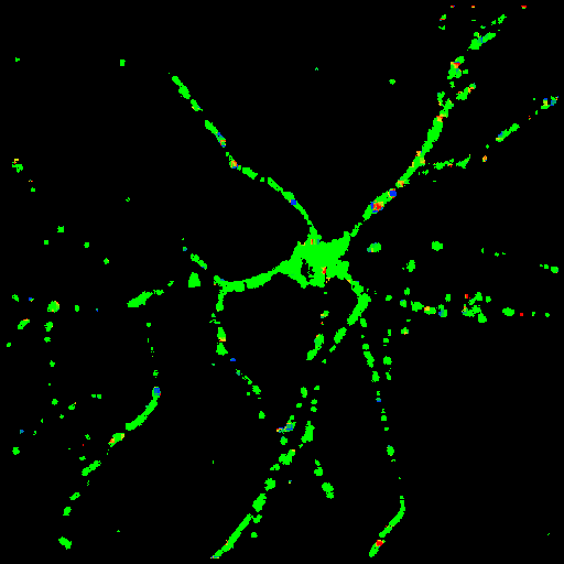
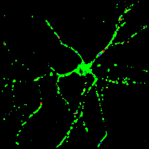
Original, minimum intensity projection image of the Optical Flow recording (GFP)	Filtered and smoothed image	Segmented Image. Each segment is marked by a different color. Use the toolbar icon to explore basic parameters of the segments by moving the mouse over the image.	Optical Flow Image
	Plot Segment Intensities for the GFP channel (Time Continuous segments=No, Constrain to active ROI=No) Each circle marks the value corresponding to and individual segment. The y-axis is scaled in fluorescence intensity.
	Plot Segment Intensities for the TMRM channel (Time Continuous segments=No, Constrain to active ROI=No)
	Plot Segment Intensities for the Optical Flow channel (Time Continuous segments=No, Constrain to active ROI=No). The y-axis is scaled in mm/sec.
		"mitochondrial segmentation wide field.ips"

Working with anterograde/retrograde motion using mean radial velocities

• If using  Multi-Dimensional Open dialog perform Optical flow loading as follows:
  • Use the point ROI tool to mark the center of the cell.
  • In the Multi-Dimensional Open dialog Processing set Optical Flow. In the Optical Flow panel set the Projection ROI parameter as number of the point ROI.
  • Set Output as Absolute value of Projected Vectors: Yes
  • Press Open.
• If using simple time lapse recordings, load the original (raw) fluorescence time lapse image sequence.
  • Use the point ROI tool to mark the center of the cell.
  • In the parameters of the Optical Flow set Output as Absolute value of Projected Vectors=Yes
  • Perform Optical Flow calculation, and Block filtering of the raw fluorescence images as detailed in the beginning of the protocol.

Original image with the point ROI in the soma	Radial velocity image (note the +/- scaling in the bottom) The y-axis is scaled in mm/sec.

Working with velocity vectors and transport/wiggling motion

• In the parameters of the Optical Flow set Output as X and Y components of vectors=Yes and Output as Absolute value of vectors=Yes
• Using Plotting/Plot Intensities Corresponding to Segments (Type=Mean, all other parameters are No) and transfer velocities corresponding to mean velocities, X and Y vector components to statistics/spreadsheet software. Working with or plotting vectors is not supported by Image Analyst MKII.
• To obtain the wiggle ratio in the statistics/spreadsheet software perform the following calculation:
  • The wiggle ratio¹ is the ratio of the mean of absolute vectors over the absolute value of the mean vector
  • So calculate first the absolute value of mean vector as SQRT(SQR(X-component)+SQR(Y-component))
  • And divide the absolute optical flow with the above result
  • This results the wiggle ratio which has a value of ~1 for linear transport movement and is larger for wiggling movement .

X component of the velocity vectors The y-axis is scaled in mm/sec.	Y component of the velocity vectors The y-axis is scaled in mm/sec.

Protocol by Akos A. Gerencser 03/07/2010 V1.0        

References

1. Gerencser A. A. and Nicholls D. G. (2008) Measurement of Instantaneous Velocity Vectors of Organelle Transport: Mitochondrial Transport and Bioenergetics in Hippocampal Neurons. Biophys J. 2008 Sep 15;95(6):3079-99.