![]()
Measurment of mitochondria to cell volume fraction
Sample preparation, reagents
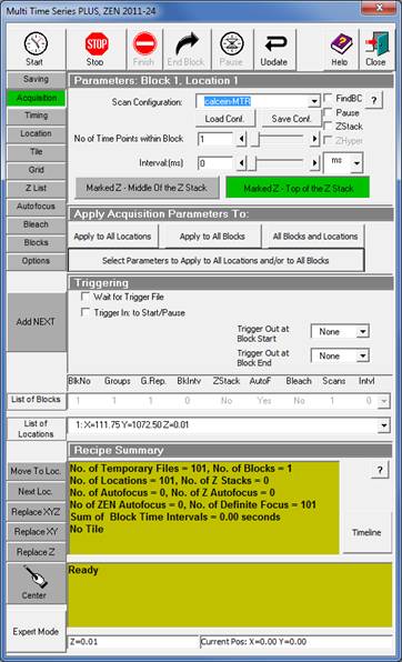
Image acquisition with Zeiss LSM780 and Zeiss LSM Multi Time Series PLUS, ZEN 2011-24 module with Definite Focus
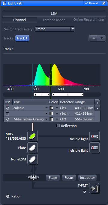
The aim is to record best possible quality, slightly oversampled images at evenly spaced z-coordinates from the bottom to the top of the culture. Due to strong photo-toxicity and photo-bleaching it is not possible to use z-stacking, but different x,y-coordinates of the culture are scanned systematically at incrementing z-coordinates. To automate this, the Zeiss LSM Multi Time Series dialogue is used with overriding Z-offset values with an Excel / Regedit trick. Microscope Settings are given below for Zeiss LSM 780, ZEN2011 software with Multi Time Series PLUS, ZEN 2011-24 module equipped with Definite Focus. Here the protocol is given for an LSM780 equipped with a spectral detector and 561nm diode laser. See 'Manual image acquisition' below if using other microscope or not having the Multi Time Lapse module.
|
|
|
|
|
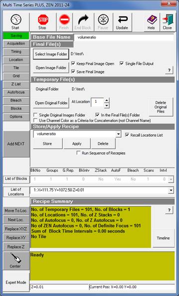
Saving tab |
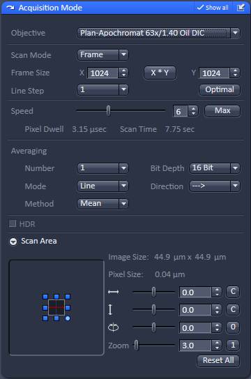
Acquisition tab |
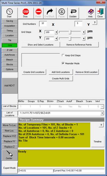
Grid tab (described below) |
|
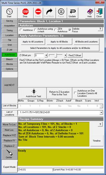
Autofocus |
Timing Tab (missing) |
Windows Registry Editor Version 5.00
[HKEY_CURRENT_USER\Software\Carl Zeiss Jena GmbH\UI\AutoTime\VolumeRatio]
[HKEY_CURRENT_USER\Software\Carl Zeiss Jena GmbH\UI\AutoTime\VolumeRatio\Block1]
1. Focus an area in the sample that is not going to be recorded.
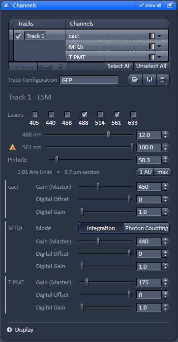
2. Set up laser powers and gains to result no saturation of images. Saturated pixels prevent accurate analysis.
3. Save the adjusted ‘calcein-MTR’ configuration.
4. In the ZEN press Locate and switch to eyepiece / transmitted light
5. If doing post-hoc immunocytochemistry, set the top edge of the well into the center of the view field, go to the Acquisition tab and zero the focus by pressing 'Manually' in the Focus panel, and zero the stage by pressing 'Set zero' in the Stage panel
6. Go back to the Multi Time Series
7. Search for a 50-100 cells under eyepiece, center each in the view field and press 'Add NEXT'.
8. Optionally cycle around all the selected cells to see that they are centered, and there are no cells imaged more than once.
9. Move to the first position
10. In the ZEN turn off 488 and set 561 laser to 5% power and using live scan focus the lowest plane where mitochondria are sharply visible. Stop scanning.
11. In the Multi Time Series, Autofocus tab, press ‘Find Z Offset’. [The offset will show zero, but the focusing is now initialized.]
12. Save the above settings in the Saving tab Store/Apply Recipe under the ‘VolumeRatio’ name. Wait until done.
13. In the Windows Explorer double click volumeratio.reg and OK to enter its contents to the system Registry.
14. Use the Store/Apply button to Apply parameters into registry under the name of “VolumeRatio”.
15. In the Acquisition tab set Scan Configuration to 'calcein-MTR': and press Apply to All Locations.
16. Verify other settings as above given in the Multi Time Series, including file name and folder.
17. Press Start.
18. If doing post-hoc immunocytochemistry, after finished imaging in the Saving tab Store the recipe under a unique name. This will store the image coordinates for later revisiting.
1. Focus an area in the sample that is not going to be recorded.
2. Set up laser powers and detector gains to result no saturation of images. Saturated pixels prevent accurate analysis.
3. Save the adjusted ‘calcein-MTR’ configuration.
4. In the ZEN press Locate and switch to eyepiece / transmitted light
5. If doing post-hoc immunocytochemistry, set the top edge of the well into the center of the view field, go to the Acquisition tab and zero the focus by pressing 'Manually' in the Focus panel, and zero the stage by pressing 'Set zero' in the Stage panel
6. Go back to the Multi Time Series
7. Select a homogeneous area of in each well to be imaged and press 'Add NEXT'.
8. Optionally cycle around all the selected wells to see that they are still in focus.
9. Optionally save the settings.
10. In the Grid tab set 10 for X and 5 for Y and 100 microns for both Grid steps. [Note that these numbers have to be entered even if they are already there by default, because the dialogue tends to take zero grid steps otherwise.]
11. Check Meander mode and press Create Multi Grids.
12. Verify that you have now 50 times the number of wells selected locations.
13. Move to the first position
14. In the ZEN turn off 488 and set 561 laser to 5% power and using live scan focus the lowest plane where mitochondria are sharply visible. Stop scanning.
15. In the Multi Time Series, Autofocus tab, press ‘Find Z Offset’. [The offset will show zero, but the focusing is now initialized.]
16. Save the above settings in the Saving tab Store/Apply Recipe under the ‘VolumeRatio’ name. Wait until done. [Note: It is important to used this configuration name for the procedure below.]
17. Adjust the number of rows in the ‘volumeratioDefiniteFocus.xls’ to match (or exceed) the number of total positions, and copy columns to the ‘volumeratio.reg’ as above described.
18. In the Windows Explorer double click ‘volumeratio.reg’ and OK to enter its contents to the system Registry.
19. Use the Store/Apply button to Apply parameters into registry under the name of “VolumeRatio”.
20. In the Acquisition tab set Scan Configuration to 'calcein-MTR': and press Apply to All Locations.
21. Verify other settings as above given in the Multi Time Series, including file name and folder.
22. Press Start.
23. Keep an eye on the microscope, checking whether the Definite Focus correctly engages as the acquisition moves from well to well. If fails reload the configuration saved in #9 and repeat from #10 using the remaining well positions.
24. If doing post-hoc immunocytochemistry, after finished imaging in the Saving tab Store the recipe under a unique name. This will store the image coordinates for later revisiting.
5. Recording post-hoc immunocytochemistry (requiring the Multi Time Series PLUS module of the Zeiss ZEN software)
1. In the ZEN load the previously defined ‘counterstain’ configuration. If not yet defined do the following:
1. load ‘calcein-MTR’ configuration, and change the Light Path and Channels to match the fluorescence of the label. Usually calcein and Mitotracker Red are washed out by this time or outshined by the staining.
2. Keep the same Acquisition mode settings, however Faster speed and Bi-directional scanning may be used.
3. Save the new configuration as ‘counterstain’ (arbitrary name).
2. Press Locate and switch to eyepiece / transmitted light and set the top edge of the well into the center of the viewfield, go to the Acquisition tab and zero the focus by pressing 'Manually' in the Focus panel, and zero the stage by pressing 'Set zero' in the Stage panel
3. Go back to the Multi Time Series and under Saving tab Store/Apply Recipe load the previously stored coordinates. [Note, that stored coordinates need to be loaded after pressing ‘Set zero’ above.]
4. In the ZEN load the live cell calcein-MTR recording. You may split the screen to see live image and the original recording in the same time.
5. In the Multi Time Series select any position and using Live scan in the ZEN, try to find the same cell compared to the live recording, by dragging the scan area in the Acquisition mode panel. [Note, that tiled acquisition is also an option to find the same cell]
6. If not finding the cell, the zero position may need to be adjusted, and coordinates re-loaded.
7. If the Live scan image matches the previously recorded calcein-MTR image, stop scanning and save the ‘counterstain’ configuration.
8. Move to the first position
9. Using live scan focus the lowest plane where the cell is sharply visible. Stop scanning.
10. In the Multi Time Series, Autofocus tab, press ‘Find Z Offset’. [The offset will show zero, but the focusing is now initialized.]
11. Save the above settings in the Saving tab Store/Apply Recipe under the ‘VolumeRatio’ name. Wait until done. [Note: It is important to use this configuration name for the procedure below.]
12. In the Windows Explorer double click the previously used ‘volumeratio.reg’ and OK to enter its contents to the System Registry.
13. Use the Store/Apply button to Apply parameters into registry under the name of “VolumeRatio”.
14. In the Acquisition tab set Scan Configuration to ‘counterstain’ and press Apply to All Locations.
15. Verify other settings as above given in the Multi Time Series, including file name and folder.
16. Press Start. [Note, if split-screen was used, you can side-be-side scroll the live-cell recording to verify the match.]
Analysis in Image Analyst MKII
Use Image Analyst MKII to determine areas corresponding to mitochondria and the whole cell by using adaptive thresholding.
This protocol assumes that the user is familiar with the following sections of the online manual:
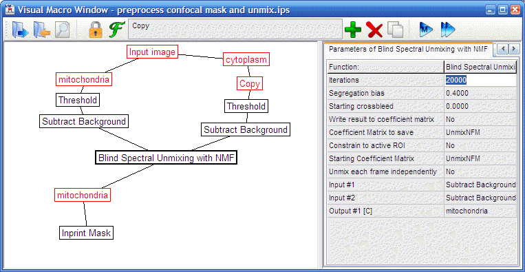
Pipelines with and without spectral unmixing
Note: for 488/561 excitation no spectral unmixing is required. For 488/543 excitation use the ‘unmix’ versions of the pipeline. This uses an adaptive spectral unmixing, based on the differential staining of mitochondria and the cytosol.
Adjustments necessary to run the pipeline
This adjustment may need to be done if using a different microscope configuration for recording than the above specified. The following steps are dependent on the bit depth of the recording:
· The pipeline discards blank images to prevent biasing intensity rescaling of the image series. Such blank frames may occur in high z-planes, or if an automatically spread grid misses any cells. The mean intensity of an image containing minimal useful information needs to be set.
· If spectral unmixing is used, the pipeline contains an algorithm to protect saturated pixels.
To adjust bit depth in the pipeline, do the following:
1. Load the pipeline
2. If this is with spectral unmixing, in the first Threshold command (captioned as Threshold: saturation) set as value: 65535 if using 16 bit or 4095 of using 12 bit recording.
3. To set value for ‘Remove blank frames’ command, perform the following procedure, if there are missed blank frames:
a. Create a 1024x1024 ROI using the Plotting/Create ROI command.
b. Press plot.
c. Find an intensity that clearly distinguishes missed, blank frames.
d. Enter this intensity value in the Value field of the ‘Remove blank frames’ command of the pipeline.
4. Save the pipeline.
Adjustment of the number of immunocytochemistry channels:
1. Load the pipeline
2. In the top right corner of the pipeline diagram add or remove channels as follows:
a. Unlock editing by clicking …
b. To remove a channel right click and delete unnecessary channel number and corresponding ‘Set scaling/LUT’ and ‘Window command’ commands below.
c. To add a channel, right click and copy-paste a channel number and corresponding ‘Set scaling/LUT’ and ‘Window command’ commands below.
i. Drop new channel number (‘Get Linked Channel’ command) on ‘Remove blank frames’ and set channel number as appears in the Multi-Dimensiona lOpen dialog
ii. Drop ‘Set scaling/LUT’ on channel number
iii. Drop ‘Window command’ on ‘Set scaling/LUT’
iv. Drop ‘Attach Overlay Image’ on ‘Set scaling/LUT’
3. Save the pipeline.
Protocol without post-hoc immunostaining
Protocol with post-hoc immunostaining
|
|
"volumeratio
preprocess confocal mask and unmix.ips" |
Tuning the pipeline
The pipeline has been originally tuned to produce similar volume fractions to electron microscopy stereology on INS-1E cells. Normally the detection of mitochondrial profiles does not have to be adjusted. However, the cytosolic staining can be quite different between cell types because of differences in confluence and presence or absence of intracellular vacuoles with very bright staining. Therefore the rescaling percentages before thresholding of the calcein image may have to be adjusted.
|
|
“volumeratio process
confocal cortical-masked.ips” |
|
|
|
|
|
|
|
|
Original Mitotracker Red image. Shown at 25% zoom. Click to see in original size. |
Original calcein image. Shown at 25% zoom. Click to see in original size. |
Hand-masked calcein image |
binarized calcein
image |
|
|
|
|
|
|
Unmixed Mitotracker Red image |
Highpass filtered Mitotracker Red image |
Binarized, masked
Mitotracker Red image |
|
The factor KV=0.667 derives from the stereologic correction formula for spheres with equal thickness to the section and truncated at half maximal intensity. Since mitochondria are thinner than the optical thickness, they are blurred by definition to the size of optical thickness, therefore the thickness of mitochondria equals to the section thickness. The correction formula (Weibel and Paumgartner 1978), where g is the relative section thickness, which is 1 (see above). r is the relative smallest visible cap section, which is 1 where objects are clipped at half maximal intensity. Therefore KV=2/3. Cells are a lot thicker than the focal plane therefore no correction factor applies for the calcein channel.
![]()
Protocol by Akos A. Gerencser 03/03/2014
V2.0 ![]()
Who to cite? We used this technology in the following papers:
Other references: